
 Technology
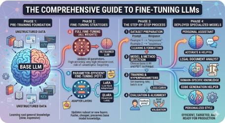
Fine-tuning is the process of taking a pre-trained language model (a large neural network that has learned general language patterns from a massive dataset) and further training it on a smaller, more specific dataset. Think of it like this:
Let’s say you have a LLM like GPT-3 that has been pre-trained on a massive dataset of internet text.
- Pre-trained Model: Can answer general questions, write creative text, summarize articles, translate languages, etc.
- Fine-tuning Goal: You want this LLM to become an expert in generating customer support responses for a specific e-commerce company, dealing with returns, shipping inquiries, and product issues.
- Fine-tuning Data: You would gather a dataset of your company’s past customer support interactions, including customer queries and the corresponding human-generated responses.
- Fine-tuned Model: After fine-tuning, the LLM will be much better at understanding customer queries specific to your company’s products and policies, and generating accurate, on-brand, and helpful responses, even using your company’s specific jargon.

The model doesn’t learn from scratch; it leverages its existing broad knowledge and adapts it to the nuances, terminology, and patterns of the new, specific domain.
Why Do We Need Fine-tuning?
Fine-tuning is crucial for several reasons:
- Pre-trained models are generalists. Fine-tuning allows them to become specialists in a particular domain (e.g., legal, medical, financial, customer service) by adapting to its specific terminology, style, and knowledge.
- While a pre-trained model might be good at general text generation, fine-tuning can make it excel at a very specific task like sentiment analysis, named entity recognition, summarization of legal documents, or generating code in a specific programming language.
- For specific tasks, a fine-tuned model almost always outperforms a general pre-trained model because it has learned to focus on the relevant patterns and information within that specific context.
- Training a large language model from scratch requires astronomical amounts of data and computational resources. Fine-tuning requires significantly less data and compute, making it a much more practical approach for most applications.
- Building a powerful, task-specific model from scratch is prohibitively expensive. Fine-tuning offers a cost-effective way to leverage existing powerful models and tailor them to specific needs.
How is Fine-tuning Different from Pre-training?
The key differences between pre-training and fine-tuning lie in their scale, objective, data, and computational cost :

- Pre-training:
a. Pre-training aims to impart broad language understanding, encompassing grammar, factual knowledge, and reasoning skills, by exposing a model to extensive and varied text data. This process typically involves unsupervised or self-supervised learning, where the model learns to predict subsequent words or complete missing ones.
b. The training data for pre-training consists of billions of words sourced from diverse online materials like books, articles, websites, and code. This data is generally unlabeled or self-labeled.
c. Pre-training commences with a model having randomly initialized weights (starting from scratch).
d. The training is conducted from the ground up, requiring substantial computational resources (thousands of GPUs) and extended periods (weeks or months). During this phase, all layers of the neural network undergo training.
e. The expense of pre-training is exceptionally high , ranging from tens to hundreds of millions of dollars.
f. Pre-training yields a versatile, general-purpose language model capable of addressing a broad spectrum of tasks. However, without further fine-tuning, it may not achieve top-tier performance in highly specialized areas.
- Fine-Tuning:
a. Fine-tuning aims to tailor a pre-trained model’s existing knowledge to excel in a specific task or domain . This process enables the model to learn a particular function, such as classification or prompt-based generation.
b. Training Data utilizes smaller, task- or domain-relevant datasets, typically containing thousands of labeled examples.
c. Model State begins with the pre-trained model’s established weights.
d. Training Process involves continued training, usually for a shorter period and with fewer computational resources. Strategies may include training only the upper layers or applying a reduced learning rate across all layers.
e. The expense of fine-tuning is relatively inexpensive , ranging from hundreds to thousands of dollars depending on data and model size.
f. A specialized model highly optimized for a defined task or domain , benefiting from the foundational knowledge of the pre-trained model.
Let’s use an analogy to understand.
- Pre-training: Learning the fundamental rules of the road, how a car works, traffic laws, and general driving techniques in a wide variety of environments (city, highway, rural roads). This is like taking a comprehensive driving course and getting your driver’s license. You can now drive a car .
- Fine-tuning: Now, you’ve been hired as a professional race car driver. You already know how to drive , but you need to specialize. This involves:
- Training on a specific race track (your fine-tuning dataset).
- Learning the nuances of a specific type of race car (adapting to specific model parameters).
- Practicing specific race maneuvers and strategies (optimizing for the specific task).
- This specialized training makes you an expert race car driver , far more proficient on the track than someone who only has a general driver’s license.
Post-Training
“Post-training” is an umbrella term encompassing all the training and refinement steps applied to a Large Language Model after its initial broad pre-training .
As we discussed, pre-training builds the foundational understanding and general knowledge. Post-training then takes this “base model” and shapes it to be more useful, aligned with human intentions, safer, and often more performant on specific tasks or domains.
The goal of post-training is to transform a raw, intelligent but unrefined LLM into a practical and reliable tool for various applications. It addresses limitations of pre-trained models such as:
- Pre-trained models might generate coherent text but struggle to follow specific commands.
- They might generate factually incorrect information.
- They can perpetuate biases present in their training data or generate harmful content.
- They might be too large or slow for real-world deployment.
- While they can generate text, their ability to perform complex, multi-step reasoning might be weak.
Different Types of Post-Training

While “fine-tuning” is a core component, post-training includes several distinct techniques, each addressing specific aspects:
- Fine-tuning (Supervised Fine-tuning — SFT):
To adapt the model to a specific task, domain, or instruction-following by training it on a relatively small, high-quality, labeled dataset of input-output pairs. This is the most common form of post-training.
It continues the supervised learning process, adjusting the model’s weights based on the provided examples.
Ex: This is like a general driver who, after getting their license (pre-training), takes additional, specialized driving lessons to become proficient in a specific type of driving, like navigating a busy city (learning city-specific rules, anticipating traffic patterns, etc.) or driving a specific type of vehicle like a truck (understanding its unique handling). The underlying driving skills are already there, but they are refined for a particular context.
2. Alignment (e.g., Reinforcement Learning from Human Feedback — RLHF, Direct Preference Optimization — DPO):
To align the model’s behavior with human preferences, values, and safety guidelines. This is crucial for making LLMs helpful, harmless, and honest. It often goes beyond just task performance to focus on the quality and appropriateness of the response.
In RLHF, human annotators rank or compare different model outputs. This human feedback is used to train a separate “reward model,” which then guides the LLM to produce outputs that are preferred by humans using reinforcement learning. DPO simplifies this by directly optimizing the LLM based on human preferences without an explicit reward model.
Ex: This is like having a driving instructor or a driving safety committee (human feedback) constantly evaluating your driving. They don’t just tell you how to drive (fine-tuning), but how to drive safely, ethically, and courteously . They might give you feedback like, “You shouldn’t speed, even if you know the route” (safety alignment), or “You should always yield to pedestrians” (ethical alignment), or “That was a good, smooth turn” (preference alignment). This feedback refines your driving style to be more socially acceptable and safe, even if you could technically complete the journey otherwise.
3. Reasoning Enhancement:
To improve the LLM’s ability to perform complex, multi-step logical reasoning, problem-solving, and chain-of-thought processes. While pre-training provides some reasoning capacity, it can be limited.
This often involves training on datasets specifically designed to teach reasoning patterns, such as mathematical problems with step-by-step solutions, logical puzzles, or code generation with explanations. Techniques like Chain-of-Thought (CoT) prompting or training on CoT datasets are key here.
Ex: This is like a driver learning advanced defensive driving techniques or tactical planning for long journeys. It’s not just about knowing how to drive (pre-training) or driving safely (alignment), but about:
- Anticipating complex situations: “If that car slows down and the light turns yellow, what are my options to avoid a sudden stop?” (multi-step problem-solving).
- Breaking down a complex route: “First, I need to get onto the freeway, then take exit 23, then turn left at the third traffic light, and finally, look for the blue mailbox.” (chain-of-thought reasoning).
- Understanding cause and effect: “If I brake suddenly on wet pavement, what will happen?” (logical deduction).
4. Efficiency Optimization:
To make the LLM smaller, faster, and more resource-efficient for deployment, especially on edge devices or in high-throughput applications. Large LLMs can be computationally expensive.
This involves techniques like:
- Quantization: Reducing the precision of the model’s weights (e.g., from 32-bit to 8-bit integers) to save memory and speed up computation.
- Pruning: Removing less important connections (weights) in the neural network.
- Knowledge Distillation: Training a smaller “student” model to mimic the behavior of a larger, more powerful “teacher” model.
- Parameter-Efficient Fine-Tuning (PEFT) methods (e.g., LoRA): Only training a small fraction of the model’s parameters during fine-tuning, significantly reducing computational cost and memory.
Ex: This is like optimizing your car for fuel efficiency and speed. You’re not changing how it drives or what it can do (its core functions), but you’re making it run smoother, use less gas, and accelerate faster. This could involve:
- Lightening the car’s weight: (pruning redundant parts of the model).
- Using more efficient engine components: (quantization for faster calculations).
- Installing a smaller, more streamlined engine that performs like a larger one: (knowledge distillation from a larger model to a smaller one).
- Fine-tuning only specific engine settings for optimal performance rather than rebuilding the entire engine: (PEFT methods like LoRA).


Types of Fine Tuning are:
1. Transfer Learning
This is a broader machine learning paradigm where a model trained on one task (the “source task”) is reused as a starting point for a different but related task (the “target task”). Fine-tuning LLMs is a prime example of transfer learning. The pre-training phase extracts vast amounts of general language knowledge (the source task), and then fine-tuning adapts this knowledge to a specific downstream task (the target task).
The entire LLM paradigm is built on transfer learning. It’s efficient because you don’t train from scratch.
- Source Task: Predicting the next word in a massive internet corpus (pre-training). This teaches the LLM grammar, semantics, world knowledge.
- Target Task: Answering medical questions.
- Process: You take an LLM pre-trained on general text (transferring its general language abilities) and then fine-tune it (supervised fine-tuning) on a dataset of medical questions and answers.
2. Supervised Fine-tuning (SFT)
This is the most common and fundamental type of fine-tuning. It involves training the pre-trained LLM on a labeled dataset of input-output pairs. The model learns to map specific inputs to desired outputs based on the provided examples. The “supervision” comes from having correct answers (labels) for each input.
For specific, well-defined tasks where you have a clear idea of the desired output for a given input. This is excellent for task-specific adaptations.
Ex: Task: Sentiment Analysis.
- Data: A dataset of customer reviews, each labeled as “positive,” “negative,” or “neutral.”
- Process: You feed the LLM review text like “The service was excellent!” and train it to output “positive.” You also feed “This product broke quickly.” and train it to output “negative.”
- Result: The fine-tuned LLM becomes highly accurate at classifying the sentiment of new, unseen reviews.
3. Few-shot Fine-tuning
This refers to the ability of large, pre-trained LLMs to learn a new task or adapt to a specific style with very few examples provided directly in the prompt (the “context window”), without any actual weight updates to the model. While sometimes conflated with actual fine-tuning (weight updates), in the context of LLMs, it primarily refers to in-context learning , where the model “learns on the fly” from the provided examples within a single inference call. If actual weight updates are involved with few examples, it falls under the PEFT umbrella.
When you have extremely limited labeled data (e.g., 1–10 examples) and the task is relatively simple or a slight variation of what the base model already knows. It’s often used for rapid prototyping or for tasks where data collection is impractical.
Ex: Task: Extracting product names from customer feedback.
Extract product names:
Review: "I love my new Acme Blender! It makes great smoothies."
Products: Acme Blender

Review: "The customer service for the SuperVac was terrible."
Products: SuperVac

Review: "My RoboMop is fantastic, but the battery life is short."
Products: RoboMop

Review: "Just bought the new Quantum Headphones. Sound quality is amazing!"
Products:
LLM Output:
Quantum Headphones
Instruction Fine-tuning
Aims to make the LLM better at following instructions and generating responses in a desired format or style. It involves training the model on datasets where inputs are formulated as instructions or prompts, paired with the desired outputs. This is often the first step in creating conversational or helpful AI assistants.
When you want your LLM to act as a conversational agent, respond to commands, generate structured output (like JSON), or adopt a specific persona. It’s crucial for improving the “user-friendliness” of an LLM.
Ex: You have a base LLM that generates generic text. You want it to answer questions in a concise, helpful, and polite manner, like a virtual assistant. You would create a dataset of prompts and desired polite answers:
Input:
“Explain photosynthesis simply.”
Output:
“Photosynthesis is how plants make their own food! They use sunlight, water, and air (carbon dioxide) to create sugars for energy and release oxygen as a byproduct. Think of them as tiny chefs using these ingredients to cook their meals!”
Input:
“List the top 3 best-selling books of 2023 in JSON format.”
Output:
{"books": [{"title": "Book A", "author": "Author X"}, {"title": "Book B", "author": "Author Y"}, {"title": "Book C", "author": "Author Z"}]}
4. Domain-Specific Fine-tuning (or Domain Adaptation)
This focuses on adapting an LLM to a particular industry, field, or area of knowledge by training it on a large corpus of unlabeled or semi-labeled text specific to that domain . The goal is to make the model more knowledgeable about the domain’s terminology, facts, and discourse style. This is often done before task-specific SFT.
When the general LLM lacks sufficient depth or accuracy in a specialized domain (e.g., law, finance, biotech) and you need it to understand and generate highly accurate, domain-specific text.
Ex: Task: Building an LLM that can accurately discuss complex financial derivatives.
- Data: Millions of financial reports, analyst call transcripts, economic journals, and financial news articles. This data is largely unstructured.
- Process: You take a base LLM and continue to pre-train it on this massive financial text corpus. The model learns the specific jargon (“yield curve,” “quantitative easing,” “futures contracts”), the typical sentence structures, and the factual relationships within the financial world. After this, you might perform SFT for a specific financial task like sentiment analysis of earnings call transcripts.
Seven-Stage Fine-Tuning Pipeline for LLM
This seven-stage process covers the entire lifecycle of developing and deploying a fine-tuned LLM. This comprehensive pipeline ensures that the fine-tuned LLM not only performs well initially but remains a valuable and adaptive asset in the long term. Let’s break down each stage with an example.

1. Dataset Preparation
This is the most critical and often the most time-consuming stage. It involves collecting, cleaning, formatting, and annotating the data that will be used for fine-tuning. The quality and relevance of this dataset directly impact the performance of the fine-tuned model. This stage may include data augmentation, deduplication, and splitting into training, validation, and test sets.
Ex:
Gather historical customer support chat logs from the e-commerce platform. This includes customer questions, their intent, and the corresponding human agent’s responses.
Remove personally identifiable information (PII), irrelevant conversational filler, spam, and badly formatted entries. Standardize greetings and closings.
Convert the raw chat logs into a structured format suitable for instruction fine-tuning. For instance:
[   {"instruction": "What is the return policy for a damaged item?",
      "output": "For damaged items, you can initiate a return within 30 days of delivery. Please visit our 'Returns & Refunds' page and follow the instructions to get a prepaid shipping label. We'll send a replacement or issue a full refund upon inspection."},
    {"instruction": "Can I track my order #XYZ123?",
     "output": "Yes, you can track your order #XYZ123 by visiting our 'Order Tracking' page and entering your tracking number. You'll see the latest shipping updates there."},
]
If the original logs don’t clearly delineate instructions and responses, human annotators might need to label these segments.
Divide the dataset into 80% for training, 10% for validation (used during training to tune hyperparameters and prevent overfitting), and 10% for final testing.
2. Model Initialization
In this stage, you select the base pre-trained LLM that you intend to fine-tune. This choice depends on factors like model size, architecture, capabilities (e.g., strong code generation vs. strong reasoning), and licensing. You load the model’s pre-trained weights, and potentially its tokenizer.
Ex: Decide on a suitable base model. For a customer support chatbot, you might choose a mid-sized open-source model like Llama 3 8B, Mistral 7B, or a similar instruction-tuned base model if you want to further specialize it. These models offer a good balance of performance and efficiency.
Load the model’s weights and its associated tokenizer from a library like Hugging Face Transformers.
from transformers import AutoModelForCausalLM, AutoTokenizer

model_name = "meta-llama/Llama-3-8b-instruct" # Or your chosen base model

tokenizer = AutoTokenizer.from_pretrained(model_name)
model = AutoModelForCausalLM.from_pretrained(model_name)
Set up any initial configurations for the model, such as enabling gradient checkpointing for memory efficiency if you plan to use full fine-tuning.
3. Training Environment Setup
This stage involves setting up the computational infrastructure and software environment necessary for training. This includes selecting appropriate hardware (GPUs), installing required libraries (PyTorch, TensorFlow, Transformers, Accelerate, PEFT), and configuring distributed training if using multiple GPUs.
Ex:
Provision a cloud GPU instance (e.g., AWS EC2 with NVIDIA A100, Google Cloud with L4 GPUs) or use a local machine with a powerful GPU (e.g., NVIDIA RTX 4090).
Install Python and create a virtual environment.
Install
torch
(or
tensorflow
),
transformers
,
accelerate
,
peft
,
bitsandbytes
(for quantization if using QLoRA),
tqdm
,
datasets
, etc.
Configure the environment variables for CUDA if necessary.
If using multiple GPUs, set up
torch.distributed.launch
or
accelerate launch
for distributed training.
Set up logging (e.g., Weights & Biases, MLflow, TensorBoard) to track training progress, loss, and evaluation metrics.

4. Partial or Full Fine-Tuning
This is the core training phase where the LLM’s parameters are adjusted based on the prepared dataset.
- Full Fine-tuning: All (or nearly all) parameters of the pre-trained model are updated. This is resource-intensive but can yield the best performance if done correctly with sufficient data.
- Partial Fine-tuning (PEFT): Only a small subset of parameters is updated, or new, smaller layers are added and trained. This is much more resource-efficient and faster, reducing the risk of catastrophic forgetting. Common methods include LoRA, QLoRA, Prefix Tuning, etc.
Ex: Given the potential size of the base model and the need for efficiency, you might choose QLoRA (Quantized LoRA) . This allows fine-tuning a large model (e.g., 8B parameters) on consumer-grade GPUs by quantizing the base model to 4-bit and only training LoRA adapters.
Define training hyperparameters like:
- Learning Rate: E.g., 2e−5
- Batch Size: E.g., 4 (per device)
- Number of Epochs: E.g., 3–5
- Optimizer: AdamW
-
LoRA Configuration:
r=16,lora_alpha=32,target_modules=["q_proj", "k_proj", "v_proj", "o_proj"]
Execute the training script, feeding the prepared training data to the model. During this process, the model learns to associate customer questions with the correct customer service responses.
# Simplified pseudo-code for LoRA training

from trl import SFTTrainer
from peft import LoraConfig

lora_config = LoraConfig(r=16, lora_alpha=32,
target_modules=["q_proj", "k_proj", "v_proj", "o_proj"], ...)

trainer = SFTTrainer(
          model=model,
          train_dataset=train_dataset,
          peft_config=lora_config,
          args=training_args,
          tokenizer=tokenizer,
          formatting_func=format_chat_example)

trainer.train()
5. Evaluation and Validation
After training, the model’s performance needs to be rigorously evaluated using unseen data (the validation and test sets) to ensure it generalizes well and meets the desired objectives. Metrics vary based on the task (e.g., accuracy, BLEU, ROUGE, perplexity, human evaluation). This stage helps identify overfitting and guides hyperparameter tuning.
Ex: Metrics:
- Automatic Metrics: While exact match is hard, you might use ROUGE scores for summarization-like aspects of responses, or BLEU for response quality, though these are often insufficient for open-ended generation.
- Human Evaluation (Crucial): Have human evaluators (e.g., internal customer service agents) assess the model’s responses on the test set for:
- Helpfulness: Does it directly answer the customer’s question?
- Accuracy: Is the information provided correct (e.g., correct return period, valid tracking link)?
- Tone: Is it polite, empathetic, and on-brand?
- Coherence: Is the response grammatically correct and easy to understand ?
- Hallucinations: Does it invent information?
Evaluate the model on the validation set periodically during training to track performance and adjust hyperparameters. After training, a final evaluation on the separate test set provides an unbiased measure of generalization.
If evaluation shows deficiencies (e.g., model still provides generic answers), you might go back to Dataset Preparation (add more diverse examples), adjust hyperparameters, or try a different fine-tuning method.
6. Deployment
Once the fine-tuned model meets performance criteria, it’s prepared for deployment into a production environment where it can serve real-world requests. This involves packaging the model, setting up APIs, and ensuring scalability and low latency.
Ex: Save the fine-tuned model weights (if using PEFT, this would be the small adapter weights plus a reference to the base model).
Deploy the model behind a REST API or a specialized serving framework (e.g., Hugging Face Inference Endpoints, NVIDIA Triton Inference Server, custom FastAPI server).
Integrate the API into the e-commerce customer support system. When a customer types a question into the chat widget, the system sends it to the fine-tuned LLM API, and the LLM’s response is displayed to the customer or used to assist a human agent.
Configure the deployment to handle expected load (e.g., auto-scaling groups, load balancers) to ensure the chatbot remains responsive during peak times.
7. Monitoring and Maintenance
After deployment, continuous monitoring is essential to track the model’s performance in a live environment, detect drift, identify new failure modes, and gather data for future improvements. Maintenance involves periodically retraining the model, updating its knowledge, and addressing new challenges. Ex:
Performance Monitoring:
- Track key metrics like response time, error rates, and the frequency of “fallback to human agent” scenarios.
- Collect user feedback (e.g., “Was this helpful? Yes/No” buttons).
- Monitor for hallucinations or inappropriate responses.
Data Drift Detection: Observe if incoming customer queries start to differ significantly from the original training data, indicating a shift in user behavior or product offerings.
Feedback Loop: Log all new customer interactions and human agent corrections/edits. This new data can be periodically reviewed, annotated, and added to the dataset for the next iteration of fine-tuning, ensuring the model stays up-to-date and continuously improves.
Scheduled Retraining: Plan for regular retraining cycles (e.g., quarterly or semi-annually) to incorporate new data, address emerging issues, and adapt to product or policy changes.
Let’s deep dive into the each stage of the fine-tuning pipeline:
Data Preparation
This stage is paramount because the quality of your data directly dictates the quality of your fine-tuned LLM. Garbage in, garbage out!
Steps Involved in Data Preparation
1. Data Collection
This is the initial step where you gather the raw data that will form your fine-tuning dataset. The sources and methods depend heavily on your specific task and domain.
Sources:
- Historical Chat Logs: Transcripts of past customer service interactions (customer questions and agent responses). This is often the primary source.
- FAQ Pages/Knowledge Bases: Structured Q&A pairs from your company’s official documentation. These can be used directly or as templates for generating more conversational data.
- Product Descriptions/Reviews: Text related to your products, which can help the model understand product-specific vocabulary and features.
- Internal Company Documents: Policies, procedures, and guidelines that dictate how customer service agents should respond.
- Synthetic Data Generation: Using a larger LLM (or even the base LLM you plan to fine-tune) to generate more instruction-response pairs based on a few seed examples or a domain-specific knowledge base. This is especially useful when real data is scarce.
Methods: API calls to internal systems, web scraping, manual collection.
2. Data Preprocessing and Formatting
Raw data is rarely in a usable format. This stage involves transforming the collected data into a clean, consistent, and structured format that the LLM can learn from. It’s about making the data uniform and model-ready.
Cleaning:
- PII Masking/Anonymization: Removing or replacing sensitive customer information (names, addresses, credit card numbers, order numbers unless explicitly needed and masked appropriately).
- Deduplication: Removing identical or near-identical chat turns or questions to avoid overfitting.
- Noise Removal: Eliminating irrelevant timestamps, system messages, emojis, or formatting inconsistencies (e.g., HTML tags from scraped data).
- Spelling and Grammar Correction: Fixing common typos or grammatical errors in customer inputs (optional, depends on whether you want the model to handle messy input).
Tokenization Compatibility: Ensuring the text is compatible with the LLM’s tokenizer (e.g., handling special characters, ensuring correct encoding).
Formatting:
- Converting conversational turns into clear instruction-response pairs.
-
Adding special tokens to delineate roles (e.g.,
[CUSTOMER],[AGENT],[INST],[/INST]) or task types. - Standardizing prompts: If a customer asks “Where’s my order?” , convert it to a consistent instruction format like “Track my order for #ORDERID” if you have a tracking system.
- Ensuring desired output format: If you want JSON output for specific queries, ensure your training data provides JSON outputs.
Truncation/Padding: Deciding on max sequence length. If a chat log is too long, deciding how to truncate it; if too short, how to pad it (usually handled by the tokenizer during training).
3. Handling Data Imbalance
Data imbalance occurs when one class or category of data is significantly more frequent than others.
In LLMs, this might mean some types of customer queries are very common (e.g.,
“Where’s my order?”
), while others are rare (e.g.,
“How do I troubleshoot my smart doorbell?”
).
If not addressed, the model might become very good at the frequent tasks but perform poorly on rare but important ones.
There are different techniques to handle this:
-
Over-sampling:
Increasing the number of samples in the minority class.
Ex: If queries about “smart doorbell troubleshooting” are rare (minority class), we can duplicate existing examples of these queries, or use techniques like SMOTE (Synthetic Minority Over-sampling Technique) to generate synthetic but similar examples of these queries. -
Under-sampling:
Reducing the number of samples in the majority class.
Ex: If “Where’s my order?” queries are overwhelmingly common, you might randomly remove some of these examples from your training set to balance it with other query types. -
Adjusting Loss Function (Class Weights):
Modifying the loss function during training to give more weight to errors made on minority classes. This encourages the model to pay more attention to correctly predicting the less frequent classes.
Ex: During training, if the model incorrectly answers a “smart doorbell troubleshooting” query, the loss for that prediction is multiplied by a higher weight than if it incorrectly answers a “Where’s my order?” query. This pushes the model to optimize for the harder, less common cases. -
Focal Loss:
A specific type of loss function designed to address extreme class imbalance, especially in dense object detection but applicable elsewhere. It down-weights the contribution of
“easy”
examples (well-classified majority class examples) and focuses more on
“hard”
examples (misclassified or rare class examples).
Ex: If the model is already very good at “Where’s my order?” , Focal Loss would reduce the penalty for getting those right, directing more of the model’s learning capacity towards improving on trickier, less common queries. -
Ensemble Methods:
Training multiple models, each potentially focusing on different aspects of the data or being trained on different subsets.
Ex: You could train one LLM specifically for common queries and another, smaller LLM for complex troubleshooting, and then combine their outputs or use a routing mechanism. Or, train multiple LLMs on different balanced subsets of the data and average their predictions. - Stratified Sampling: When creating training, validation, and test sets, ensuring that the proportion of different classes is maintained across all splits. This is crucial for balanced evaluation, not just for training data itself.
-
Data Cleaning:
While not a technique
for
imbalance directly,
thorough data cleaning can implicitly help with imbalance.
If rare but important classes are buried in noise or mislabeled, cleaning makes them visible and usable, essentially
“increasing”
their effective presence.
Ex: Ensuring all “damaged item return” queries are consistently labeled as such.
4. Splitting Dataset
After preparing your data, you must divide it into distinct subsets:
- Training Set: Used to train the model, where it learns patterns.
- Validation Set: Used during training to monitor performance, tune hyperparameters, and detect overfitting. The model does not train on this data.
- Test Set: Used only once at the very end to evaluate the final, trained model’s performance on unseen data. This provides an unbiased estimate of how well the model will perform in the real world.
There are different techniques to handle this:
-
Random Sampling:
The simplest method. Data points are randomly assigned to training, validation, and test sets.
Ex: You have 10,000 instruction-response pairs. You randomly select 8,000 for training, 1,000 for validation, and 1,000 for testing. - Stratified Sampling: Ensures that the proportion of different classes or categories is maintained across all splits (training, validation, test). This is crucial for imbalanced datasets.
-
Ex:
If 5% of your customer queries are about
“returns for damaged items,”
stratified sampling ensures that approximately
5% of your training set, 5% of your validation set, and 5% of your test set are also “returns for damaged items ” queries.
This guarantees that each split is representative of the overall data distribution. -
K-Fold Cross-Validation:
The dataset is divided into ‘k’ equal-sized folds. The model is then trained ‘k’ times. In each iteration, one fold is used as the validation/test set, and the remaining ‘k-1’ folds are used for training. The final performance is the average of the ‘k’ evaluation scores.
Ex: For our 10,000 examples, with 5-fold cross-validation:
Fold 1: Test on 2,000 examples, train on 8,000.
Fold 2: Test on different 2,000 examples, train on different 8,000.
…and so on for 5 iterations. -
Leave-One-Out Cross-Validation (LOOCV):
An extreme case of K-Fold where ‘k’ equals the number of data points. In each iteration, one single data point is used as the test set, and all others are used for training.
Ex: If you have 10,000 examples, you train the model 10,000 times, each time leaving out one example for testing.
There are existing and potential research methodologies
1. Data Annotation
Data annotation is the process of labeling or tagging raw data to add meaningful information or context. For LLMs, this often means assigning labels to text segments, classifying entire texts, or structuring unstructured text into desired input-output pairs. It’s essentially teaching the model what to look for or what to produce by providing explicit examples. This process often involves human annotators due to the complexity and nuance of language. This is important for LLMs due to :
- Supervised Learning: Most fine-tuning SFT relies heavily on annotated data. You need examples of desired inputs and outputs for the model to learn from.
- Task Specialization: If you want your LLM to perform sentiment analysis, you need text labeled with sentiment. If you want it to extract entities, you need text with entities marked.
- Alignment: For techniques like RLHF, human annotators provide the “human feedback” by rating or ranking model outputs, which is a form of annotation.
Ex: For Instruction Fine-tuning:
A customer chat log:
“Hi, I ordered a widget last week, order #12345.
It still hasn’t arrived. Can you help?”
A human annotator would read this and transform it into an instruction-response pair, perhaps following a specific internal guideline for how the chatbot should handle such queries:
Annotated Input (Instruction): “Track my order #12345, it hasn’t arrived yet.”
Annotated Output (Response): “I see your order #12345 placed on [Date]. It’s currently in transit and expected to arrive by [Estimated Date]. You can track its live status at [Tracking Link].”
For Intent Classification:
Customer query:
“What’s your policy on returning an item after 60 days?”
A human annotator assigns a label:
Return_Policy_Inquiry
.
Customer query:
“My Bose headphones arrived broken.”
A human annotator assigns a label:
Damaged_Item_Report
.
For Dialogue State Tracking:
A multi-turn conversation.
Mark down what pieces of information (slots) the customer has provided (e.g.,
product_type: headphones
,
issue: broken
).
2. Data Augmentation
Data augmentation is the process of artificially increasing the size and diversity of a training dataset by creating modified versions of existing data. For text, this means generating new text samples that are variations of the original, without changing their core meaning or label. It helps prevent overfitting and improves the model’s generalization capabilities. This stage is important for LLMs for few reasons:
- Real-world annotated data can be expensive and time-consuming to obtain. Augmentation provides more training examples from limited initial data.
- By exposing the model to slightly different phrasings, synonyms, or grammatical structures, it becomes more resilient to variations in user input.
- A larger, more diverse dataset helps the model learn generalizable patterns rather than memorizing specific examples.
There are different techniques of Text Data Augmentation:
-
Synonym Replacement:
Replacing words with their synonyms
Ex: “fast” -> “quick”. - Random Insertion/Deletion/Swap: Randomly inserting irrelevant words, deleting words, or swapping adjacent words (with careful consideration to maintain meaning).
-
Back Translation:
Translating text from its original language to another language and then back to the original. This often introduces natural linguistic variations.
Ex: English -> Spanish -> English:
Original: “Can I get a refund for my order?”
Spanish: “¿Puedo obtener un reembolso por mi pedido?”
Back-translated English: “Can I receive a reimbursement for my order?” (Slightly different phrasing, same meaning). -
Paraphrasing:
Rewriting sentences or phrases to express the same meaning in different words. This is where LLMs themselves become very useful.
Ex:
Original: “My package hasn’t arrived. What’s the status?”
Paraphrase 1: “I’m still waiting for my delivery. Can you check its whereabouts?”
Paraphrase 2: “Could you please give me an update on my missing shipment?” - Noise Injection: Adding typos or grammatical errors to make the model more robust to imperfect user input.
3. Synthetic Data Generation using LLMs
This is a powerful and increasingly popular method where you leverage existing, often larger, pre-trained LLMs to generate entirely new data that mimics the characteristics of your target domain or task. Instead of just transforming existing data (augmentation), you’re creating new data points from scratch, often based on a few seed examples or a descriptive schema. This stage is important for LLMs for few reasons:
- Rapidly generate large volumes of data when human annotation is too slow or expensive.
- Can help generate diverse examples that might be missing from real-world data, including edge cases or specific scenarios.
- Reduces reliance on expensive human annotators for bulk data creation.
- You can prompt the LLM to generate data specifically for certain difficult scenarios or underrepresented classes.
There are different techniques to manage this:
-
Prompting:
Provide the LLM with a template or specific instructions on how to generate input-output pairs.
Ex: You give a powerful LLM (e.g., GPT-4, or even the base LLM you’re fine-tuning, if it’s capable) a few seed examples of return policy questions.
Prompt: “Generate 10 diverse customer questions related to returning items, including different reasons for return (wrong size, damaged, unwanted) and different items (clothes, electronics, books).”
LLM Output:
“I need to return this dress because it’s too small. How do I do that?”
“My new laptop arrived with a cracked screen. What’s the process for getting a replacement?”
“I bought a novel as a gift, but they already have it. Can I return it?”
… and 7 more variations …
You then pair these with existing valid answers or have a human quickly generate/verify answers for the new questions.
- Self-Instruct: An LLM generates instructions and then provides responses to those instructions, potentially filtered and refined by human review.
-
Role-Playing/Dialogue Generation:
Prompting an LLM to act as a customer and another LLM (or the same one with a different persona) to act as an agent, simulating conversations.
Ex: You might prompt the LLM with a product name and a common issue, asking it to generate a detailed troubleshooting question:
Prompt: “Imagine a customer is having trouble with their ‘SmartPlug Pro’. Generate a detailed, multi-step troubleshooting question they might ask, assuming they’ve tried basic resets.”
LLM Output (customer instruction): “My SmartPlug Pro isn’t connecting to my Wi-Fi despite resetting it multiple times and moving it closer to the router. The indicator light just blinks green, but it never goes solid. What specific network settings should I check on my router, or could there be an issue with my device’s firmware?”
A human (or another specialized LLM) would then provide the ideal answer.
Important Considerations for Synthetic Data:
- Synthetic data must be carefully reviewed and filtered. LLMs can “hallucinate” or generate repetitive/low-quality examples if not constrained.
- The LLM generating synthetic data needs to be sufficiently aligned with your target domain to produce relevant and accurate data.
- Use synthetic data to fill gaps and balance datasets, not to completely replace real-world data. A mix often yields the best results.
Let’s move on to the Model Initialization stage.
Model Initialization
This is where you prepare your chosen LLM to be ready for the fine-tuning process.
Steps Involved in Model Initialization

1. Set Up the Environment:
Before you do anything else, you need a clean and organized workspace. This involves creating a dedicated directory for your project and setting up a virtual environment. Virtual environments ensure that your project’s dependencies don’t conflict with other Python projects on your system.
Ex:
Creating a project directory:
mkdir ecom_chatbot_finetune
cd ecom_chatbot_finetune
Creating and activating a virtual environment:
python -m venv venv_ecom_chatbot
source venv_ecom_chatbot/bin/activate
2. Install the Dependencies:
Once your environment is set up, you need to install all the necessary Python libraries that your fine-tuning script will use. These include libraries for interacting with LLMs, managing data, and optimizing the training process. It’s good practice to list these in a
requirements.txt
file for reproducibility.
Ex: Sample
requirements.txt
:
torch>=2.0.0
transformers>=4.38.0
datasets>=2.18.0
accelerate>=0.28.0
peft>=0.9.0
bitsandbytes>=0.43.0
trl>=0.8.0
scikit-learn>=1.4.0
Installation Command :
pip install -r requirements.txt
3. Import the Libraries:
In your Python script, you’ll need to explicitly import the modules and classes you plan to use from the installed libraries. This makes their functionalities available within your code.
import torch from transformers
import AutoModelForCausalLM, AutoTokenizer, BitsAndBytesConfig
from datasets import load_dataset
from peft import LoraConfig, get_peft_model, prepare_model_for_kbit_training
from trl import SFTTrainer

import os
import logging
4. Choose the Language Model:
This is the crucial decision point where you select the specific pre-trained LLM that will serve as the base for your fine-tuning. Considerations include:
- Size: Larger models are more capable but require more resources.
-
Architecture:
Transformer-decoder only (like GPT, Llama) for generation, or
encoder-decoder (like T5, BART) for sequence-to-sequence tasks. - Base vs. Instruction-tuned: A “base” model is raw, while an “instruction-tuned” model has already undergone some SFT or RLHF to follow commands. For further specialization, starting with an instruction-tuned model is often beneficial.
- Licensing: Open-source (Apache 2.0, MIT) vs. proprietary (Meta Llama 3, Google Gemma).
- Community Support/Benchmarks: Popular models have more resources and better documentation.
Ex:
You decide to use
meta-llama/Llama-3-8b-instruct
. This is a relatively powerful yet manageable model size, and the
instruct
version means it already has some instruction-following capabilities, which is a good starting point for a chatbot.
model_id = "meta-llama/Llama-3-8b-instruct"
5. Download the Model from the Repository:
After choosing your model, you need to download its pre-trained weights and associated tokenizer files. Hugging Face’s
transformers
library simplifies this by automatically downloading them from the Hugging Face Hub (a vast repository of pre-trained models).
Ex:
The
AutoTokenizer.from_pretrained()
and
AutoModelForCausalLM.from_pretrained()
functions handle the download automatically if the model isn't cached locally.
# Load tokenizer
tokenizer = AutoTokenizer.from_pretrained(model_id)
tokenizer.pad_token = tokenizer.eos_token

# Configure quantization for QLoRA if desired (for efficiency)
bnb_config = BitsAndBytesConfig(
                  load_in_4bit=True,
                  bnb_4bit_quant_type="nf4",
                  bnb_4bit_compute_dtype=torch.bfloat16,
                  bnb_4bit_use_double_quant=True, )

# Load model with quantization
model = AutoModelForCausalLM.from_pretrained(
               model_id,
               quantization_config=bnb_config,
               device_map="auto" )

# Prepare model for k-bit training (essential for QLoRA)
model = prepare_model_for_kbit_training(model)
6. Load the Model in the Memory:
Once downloaded, the model’s weights need to be loaded into your computer’s memory, specifically into the GPU’s VRAM if you’re using a GPU for training. This step makes the model accessible for computations. The
device_map="auto"
argument in
transformers
helps manage this across multiple GPUs.
Ex:
AutoModelForCausalLM.from_pretrained()
function, especially with
device_map="auto"
, handles loading the model directly into the appropriate memory (CPU or GPU VRAM).
For PEFT methods like LoRA, after loading the base model, you then wrap it with the PEFT model to initialize the trainable adapters.
# Define LoRA configuration

lora_config = LoraConfig(r=16,lora_alpha=32,
            target_modules=["q_proj", "k_proj", "v_proj", "o_proj", "gate_proj", "up_proj", "down_proj"],
            lora_dropout=0.05, bias="none", task_type="CAUSAL_LM" )  # Apply LoRA to the base model

model = get_peft_model(model, lora_config)
model.print_trainable_parameters()
Output might look like:
trainable params: 41,943,040 || all params: 8,073,506,816 || trainable%: 0.5194936453676231
(showing only a small percentage of trainable parameters with LoRA).
7. Execute Tasks:
After initialization, the model is ready to be used. This stage involves verifying that the loaded model can perform basic tasks (inference) and then proceeding to the primary goal: fine-tuning.
Ex:
Before fine-tuning, you might run a quick inference to see the base model’s default behavior.
# Simple test before fine-tuning

prompt = "User: What is your return policy?"
input_ids = tokenizer(prompt, return_tensors="pt").to("cuda") # Send to GPU

# Generate a response from the base model
with torch.no_grad():
   output = model.generate(**input_ids, max_new_tokens=100)
   print("Base Model Response:", tokenizer.decode(output[0],
         skip_special_tokens=True))
Once you confirm the model is loaded and responding, you’d integrate it into your training loop (Stage 4: Partial or Full Fine-Tuning) using your prepared dataset.
Let’s proceed to the Training Environment Setup stage,
Training Environment Setup
This is crucial for controlling how your LLM learns during fine-tuning. This stage is about configuring the “engine” of your training process.
Steps Involved in Training Setup
1. Setting up the Training Environment
While we touched on installing dependencies and loading the model earlier, “Setting up the Training Environment” also refers to configuring how the training process itself will run. This includes decisions about hardware utilization (e.g., single vs. multi-GPU), mixed precision training for efficiency, and logging.
Ex: If you have multiple GPUs, you’d use tools like Hugging Face
accelerate
to distribute the model and data across them. This is often done via a command-line utility.
accelerate launch --num_processes 4 your_finetune_script.py
Utilizing
torch.float16
or
torch.bfloat16
for computations, which can significantly speed up training and reduce memory usage without much loss in accuracy. This is often handled automatically by
accelerate
or
bitsandbytes
.
2. Defining the Hyperparameters
Hyperparameters are settings that control the learning process itself, rather than being learned by the model from the data. They are set before training begins and significantly influence the model’s performance and convergence. Getting them right is often an iterative process.
Lets take a look at Key Hyperparameters:
-
Learning Rate (LR):
This is arguably the most critical hyperparameter. It determines the
size of the steps
taken during gradient descent to update the model’s weights.
A high learning rate can cause the model to overshoot the optimal solution, leading to unstable training. A very low learning rate can make training too slow or get stuck in local minima. Learning rate schedulers (e.g., linear decay, cosine annealing) are often used to dynamically adjust the LR during training.
Ex: For fine-tuning LLMs with PEFT, a common starting point for LR is around 2e−5 (0.00002) or 5e−5 (0.00005).
If the loss isn’t decreasing, or it’s oscillating wildly, you might adjust it. -
Batch Size:
The number of training examples processed at once before the model’s weights are updated.
Larger batch sizes provide a more accurate estimate of the gradient but require more memory.
Smaller batch sizes introduce more noise into the gradient updates but can sometimes lead to better generalization and fit into less VRAM.
Ex: Due to LLM size, batch sizes are often small (e.g., 1, 2, 4, 8) per GPU. Techniques like gradient accumulation can simulate larger effective batch sizes by summing gradients over several mini-batches before updating weights. -
Epochs:
One epoch means that the entire training dataset has been passed forward and backward through the neural network exactly once. The
number of epochs
determines how many times the model will see the entire dataset.
Too few epochs can lead to underfitting (model hasn’t learned enough), while too many can lead to overfitting (model memorizes training data but performs poorly on new data). - Ex: For fine-tuning LLMs, 1–5 epochs is a common range, especially with large datasets or when using PEFT, as the model starts with strong pre-trained knowledge.
Automated Hyperparameter Tuning:
Manually finding optimal hyperparameters is tedious and time-consuming. Automated methods systematically search the hyperparameter space to find combinations that yield the best performance.
-
Random Search:
Randomly samples hyperparameter values from predefined ranges or distributions.
Ex: Instead of trying LR values 1e−5,2e−5,3e−5,
you might randomly pick 2.3e−5,4.7e−5,1.1e−5.
Surprisingly effective, as not all hyperparameters are equally important, and random search can explore broader regions. -
Grid Search:
Exhaustively tries every possible combination of hyperparameters from a predefined set of values.
Ex: If LR can be {1e−5,2e−5} and Batch Size can be {2,4},
Grid Search will try (1e-5, 2), (1e-5, 4), (2e-5, 2), (2e-5, 4). -
Bayesian Optimization:
A more intelligent approach that builds a probabilistic model of the objective function (e.g., validation loss) based on previous evaluations. It then uses this model to intelligently choose the next hyperparameter combination to try, balancing exploration (trying new areas) and exploitation (refining promising areas).
Ex: After trying a few LR and batch size combinations, Bayesian Optimization suggests the next combination to try based on which settings it predicts will yield the biggest improvement.
Tools like Optuna or Weights & Biases Sweeps often use this.
3. Initializing Optimizers and Loss Functions: These are core components of the training algorithm that dictate how the model learns from errors.
-
Loss Function:
A mathematical function that quantifies the
“error”
or “distance” between the model’s predictions and the true target values.
The goal of training is to minimize this loss.
For LLMs, it’s typically a form of cross-entropy loss because they are performing next-token prediction (a multi-class classification problem for each token).
Ex: For our chatbot, the loss function would calculate how far off the model’s predicted next token is from the actual next token in the human-generated response.
If the model predicts “return” when the human said “refund,” the loss function registers an error. - Optimizers: Algorithms that adjust the model’s weights based on the gradients (the slope of the loss function) to minimize the loss. They determine the “strategy” for navigating the complex loss landscape. There are several methods:
- Gradient Descent (GD): Computes gradients over the entire dataset for each update. Impractical for large datasets like LLMs due to memory and computation.
- Stochastic Gradient Descent (SGD): Computes gradients and updates weights based on one single example at a time. Very noisy updates.
- Mini-batch Gradient Descent: A compromise between GD and SGD. Computes gradients and updates weights based on a small batch of examples (your defined batch size). This is the standard for deep learning.
-
Adaptive Optimizers:
These are more advanced optimizers that adapt the learning rate for each parameter individually based on its historical gradients.
They generally converge faster and achieve better results than vanilla SGD for deep learning.
Adam (Adaptive Moment Estimation): Combines ideas from RMSprop and AdaGrad.
It stores an exponentially decaying average of past squared gradients (vt) and an exponentially decaying average of past gradients (mt). It’s a very popular default.
AdamW: A variant of Adam that correctly implements weight decay regularization. Weight decay is crucial for preventing overfitting, especially in large models. This is the most common optimizer for LLM fine-tuning.
from transformers import TrainingArguments  # Define training arguments including optimizer
training_args = TrainingArguments(output_dir="./results",
                num_train_epochs=3,
                per_device_train_batch_size=4,
                gradient_accumulation_steps=8, # Simulate batch size of 32 (4 * 8)
                optim="adamw_8bit", # Use 8-bit AdamW for efficiency with QLoRA
                learning_rate=2e-5, logging_dir="./logs", logging_steps=100,
                evaluation_strategy="epoch", save_strategy="epoch",
                load_best_model_at_end=True,  )

# SFTTrainer will use these args to set up the optimizer and loss
# trainer = SFTTrainer(...)
Fine-Tuning the LLM
This is where the actual learning and adaptation take place. Let’s break down each step in this crucial stage.
Steps Involved in Fine-Tuning
1. Initialize the Pre-Trained Tokenizer and Model:
This step, as discussed in “Model Initialization,” is the prerequisite for fine-tuning. You load the pre-trained LLM and its corresponding tokenizer into memory. The tokenizer is essential for converting your text data into numerical tokens that the model understands, and for converting the model’s numerical outputs back into human-readable text. The model itself is loaded with its general pre-trained weights.
from transformers import AutoModelForCausalLM, AutoTokenizer, BitsAndBytesConfig
import torch

model_id = "meta-llama/Llama-3-8b-instruct"
tokenizer = AutoTokenizer.from_pretrained(model_id)
tokenizer.pad_token = tokenizer.eos_token

# For QLoRA (recommended for 8B models on consumer GPUs)
bnb_config = BitsAndBytesConfig(
    load_in_4bit=True,
    bnb_4bit_quant_type="nf4",
    bnb_4bit_compute_dtype=torch.bfloat16,
    bnb_4bit_use_double_quant=True,
)

model = AutoModelForCausalLM.from_pretrained(
    model_id,
    quantization_config=bnb_config,
    device_map="auto"
)

# Prepare model for k-bit training
from peft import prepare_model_for_kbit_training
model = prepare_model_for_kbit_training(model)
2. Modify the Model’s Output Layer:
For some
fine-tuning tasks
, especially classification or specific structured output tasks, you might need to add or modify the final layer of the pre-trained model.
For general
text generation tasks
(like chatbot, which is a form of next-token prediction), the existing output layer (the language modeling head) is usually sufficient and doesn’t need explicit modification; it’s just fine-tuned along with the rest of the model.
However, for a
classification
task (e.g., sentiment analysis), you’d replace the language modeling head with a classification head.
Ex:
If our chatbot also had to classify the
type
of customer query (e.g.,
returns
,
shipping
,
technical
), we would add a new linear layer on top of the LLM's final hidden state, with an output dimension equal to the number of query types.
Scenario where it IS needed: If you were using the LLM as a feature extractor for a separate classification task.
# This is conceptual for adding a classification head
model.classifier = torch.nn.Linear(model.config.hidden_size, num_classes)
3. Choose an Appropriate Fine-Tuning Strategy:
This is where you decide how you’re going to update the model’s weights. The choice depends on your computational resources, data size, and the specific goal (task vs. domain adaptation).
-
Task-Specific Fine-Tuning (Supervised Fine-Tuning — SFT):
Training the model on labeled input-output pairs to directly learn a specific function or behavior. This is what we’re primarily doing for our chatbot.
Ex: Training the LLM oncustomer_query -> ideal_agent_responsepairs. -
Domain-Specific Fine-Tuning (Continued Pre-training):
Further pre-training the model on a large corpus of
unlabeled
text specific to your domain to enhance its knowledge and fluency within that niche. This is often done
before
task-specific fine-tuning.
Ex: Training the LLM on all available e-commerce product manuals, internal policy documents, and customer review archives before instruction fine-tuning. -
Parameter-Efficient Fine-Tuning (PEFT):
A family of techniques (LoRA, QLoRA, Prompt Tuning) that freeze most of the base model’s parameters and only train a small, additional set of parameters. This drastically reduces computation, memory, and storage requirements.
Highly recommended for LLM fine-tuning.
Ex: For our 8B Llama 3 model, we will almost certainly use QLoRA to make it feasible on a single powerful GPU or a modest cloud instance. This involves adding small trainable LoRA adapters to the model. -
Half Fine-Tuning (HFT):
This term isn’t as standardized as the others, but it typically refers to a selective form of full fine-tuning where only a subset of the model’s layers (often the last few layers, or specific modules) are unfrozen and trained, while the earlier layers (which capture more general features) remain frozen. It’s a compromise between full fine-tuning and PEFT.
Ex: Unfreezing only the last 2–4 transformer blocks of our Llama 3 model and fine-tuning only those layers.
4. Set Up the Training Loop
This is where you bring together your data, model, optimizer, and loss function to actually run the training process. The training loop iterates over your dataset, calculates the loss, computes gradients, and updates the model’s weights.
Ex:
Using the
trl
library's
SFTTrainer
(Supervised Fine-Tuning Trainer) significantly simplifies this. It wraps the core training loop, handling aspects like gradient accumulation, mixed precision, and logging.
from trl import SFTTrainer
from transformers import TrainingArguments
from datasets import Dataset # Assuming your data is loaded into a Hugging Face Dataset

# Assume 'formatted_dataset' is your prepared data loaded into a Hugging Face Dataset
# and split into train_dataset, eval_dataset

# Function to format examples for the model's input
def formatting_func(example):
    text = f"User: {example['instruction']}\nAgent: {example['output']}"
    return {"text": text}

# Define training arguments (hyperparameters)
training_args = TrainingArguments(
    output_dir="./chatbot_results",
    num_train_epochs=3,
    per_device_train_batch_size=4,
    gradient_accumulation_steps=8, # Effective batch size 32
    optim="paged_adamw_8bit", # Optimizer optimized for 8-bit training
    learning_rate=2e-5,
    logging_dir="./chatbot_logs",
    logging_steps=10,
    evaluation_strategy="epoch", # Evaluate at the end of each epoch
    save_strategy="epoch",       # Save checkpoint at the end of each epoch
    load_best_model_at_end=True, # Load the best model based on eval metric
    fp16=False, # Set to True if your GPU supports FP16, bfloat16=True for BF16
    bf16=True,  # Set to True if your GPU supports BF16
    push_to_hub=False, # Set to True to push model to Hugging Face Hub
)

# Initialize the SFTTrainer
trainer = SFTTrainer(
    model=model,
    train_dataset=train_dataset, # Your training dataset
    eval_dataset=eval_dataset,   # Your validation dataset
    peft_config=lora_config,     # Your LoRA config from Step 1
    args=training_args,
    tokenizer=tokenizer,
    formatting_func=formatting_func, # Function to format data for input
    max_seq_length=1024, # Max context length for your model
)

# Start training!
trainer.train()
5. Incorporate Techniques for Handling Multiple Tasks (If applicable)
If your fine-tuned LLM needs to perform several distinct tasks (ex: answer FAQs, summarize returns, generate product recommendations) within the same model, you might use advanced strategies. This is less about the core training loop and more about model architecture or management.
- Fine-tuning with Multiple Adapters: Instead of one LoRA adapter, you train separate LoRA adapters for each task. At inference, you load the base model and swap in the relevant adapter for the task at hand.
-
Leveraging Mixture of Experts (MoE) Architectures:
If your base model is an MoE (like Mixtral), it’s already designed to activate different “expert” sub-networks for different inputs. Fine-tuning can further specialize these experts. For a non-MoE model, you might fine-tune different parts of the model for different tasks.
Ex: Your chatbot needs to not only answer questions but also
(a) generate a short summary of a complex return request, and
(b) translate customer feedback from Spanish to English.
You could train three separate LoRA adapters on the same base model : one for general Q&A,
one for summarization, and
one for translation.
During deployment, the system would identify the user’s intent and load the appropriate LoRA adapter on the fly.
6. Monitor Performance on a Validation Set
While training, it’s crucial to regularly evaluate the model’s performance on a separate validation set (data it has never seen during training). This helps you:
- Track Progress: See if the loss is decreasing and metrics are improving.
- Detect Overfitting: If training loss continues to decrease but validation loss starts to increase, the model is memorizing the training data and not generalizing.
- Guide Hyperparameter Tuning: Adjust learning rate, epochs, etc., based on validation performance.
We can utilize Advanced Monitoring Tools:
- Weights & Biases (W&B): Excellent for comprehensive experiment tracking, visualizing metrics, hyperparameter sweeps, and artifact management.
- TensorBoard: Google’s visualization tool for TensorFlow and PyTorch, useful for graphs and logs.
- MLflow: An open-source platform for managing the machine learning lifecycle, including experiment tracking.
Ex:
As shown in the
TrainingArguments
,
evaluation_strategy="epoch"
will trigger evaluation at the end of each epoch.
You would integrate W&B (e.g.,
pip install wandb
, then
wandb.login()
) to log training and validation loss, custom evaluation metrics (e.g., a simple accuracy if using a custom metric function, or ROUGE scores for summarization).
You’d look at the W&B dashboard to see if your
eval_loss
is consistently decreasing or if it starts to creep up, signaling overfitting.
7. Optimize Model Using Advanced Techniques / Prune and Optimize / Continuous Evaluation and Iteration
These steps are often post-training refinements or ongoing processes.
Optimise Model Using Advanced Techniques (Alignment):
-
Proximal Policy Optimization (PPO):
A reinforcement learning algorithm commonly used in
RLHF
to align LLMs with human preferences.
After SFT, a reward model is trained on human feedback, and PPO uses this reward model to further fine-tune the LLM to generate preferred responses. -
Direct Preference Optimization (DPO):
A newer, simpler alternative to PPO for alignment. It directly optimizes the LLM based on pairwise human preferences without needing an explicit reward model.
Ex: After initial instruction fine-tuning, your chatbot might be accurate but sometimes generates verbose or slightly robotic answers. You’d collect human preferences (e.g., “Response A is better than Response B”) and use DPO or RLHF to further fine-tune the model, making its responses more natural, concise, and helpful.
Prune and Optimize the Model (if necessary):
Techniques to reduce the model’s size and improve inference speed without significant performance loss. This is crucial for deployment, especially on edge devices or in high-throughput low-latency scenarios.
- Quantization (reducing numerical precision, often done during fine-tuning like QLoRA),
- Pruning (removing less important weights/neurons)
- Knowledge Distillation (training a smaller “student” model to mimic a larger “teacher” model).
Ex: Even after QLoRA fine-tuning, if the model is still too large for a specific deployment environment (e.g., a mobile app), you might further quantize it to 4-bit (if not already), or explore pruning less critical connections.
Continuous Evaluation and Iteration:
Fine-tuning is rarely a one-shot process. Models degrade over time as data distributions change or new tasks emerge. This involves setting up a feedback loop from deployment, gathering new data, and periodically retraining the model.
Ex: Regularly collect new customer queries and agent responses from the live system. Analyze common failure points of the deployed chatbot. Add new types of queries (e.g., about newly launched products, or seasonal promotions) to your dataset. Re-fine-tune the model with this updated data to keep it current and improving.
Parameter-Efficient Fine-Tuning (PEFT)
We use PEFT primarily to overcome the immense computational and memory challenges associated with fine-tuning LLMs. Training an LLM from scratch or even performing “full fine-tuning” (updating all parameters) requires:
- Massive Computational Resources: Dozens or hundreds of high-end GPUs (e.g., A100s, H100s) for weeks or months, costing millions of dollars.
- Enormous Memory Footprint: Storing the model weights, gradients, and optimizer states for billions of parameters consumes vast amounts of GPU VRAM.
- Catastrophic Forgetting: Full fine-tuning on a small, specific dataset can cause the model to “forget” much of its general knowledge acquired during pre-training, leading to degraded performance on broader tasks.
- Slow Iteration Cycles: The sheer time and cost involved in each full fine-tuning run make experimentation and iteration very slow.

PEFT methods address these issues by freezing most of the pre-trained LLM’s parameters and only training a small, additional set of parameters or making minor modifications to the model architecture . This leads to:
- Significantly Reduced Computational Cost: Trainable parameters drop from billions to millions or even thousands.
- Lower Memory Consumption: Less VRAM is needed for weights, gradients, and optimizer states.
- Faster Training: Shorter training times due to fewer computations.
- Prevention of Catastrophic Forgetting: The frozen backbone retains its general knowledge.
- Storage Efficiency: The fine-tuned “adapters” are tiny, allowing easy storage and swapping of different fine-tuned versions on a single base model.
PEFT methods can be broadly categorized based on where and how they introduce trainable parameters.
1. Prompt Modifications (Soft Prompt Tuning):
These methods modify the model’s input or activations by adding trainable vectors, effectively “prompting” the frozen LLM to perform specific tasks. The base model’s weights remain entirely frozen.
-
Soft Prompt Tuning (or simply Prompt Tuning):
Instead of using discrete, human-readable prompt tokens, soft prompt tuning prepends a small sequence of
learnable continuous vectors
(the “soft prompt”) to the input embeddings of the model. These vectors are trained via backpropagation to optimize for the downstream task. The model’s original parameters remain frozen.
Ex: For a sentiment analysis task, you’d prepend a trainable vector sequence to the embedding of “I love this product!” The LLM learns to interpret this vector sequence to produce a positive sentiment output. You don’t see discrete “tokens” for the soft prompt; it’s purely numerical.
Key Distinction of Soft Prompt vs. Prompting: -
Prompting (Hard Prompting/In-Context Learning):
Using natural language text directly in the input to guide the LLM’s behavior
Ex: “Translate this to French: …”,
“Summarize the following: …”
No training involved; relies solely on the pre-trained model’s ability to follow instructions. - Soft Prompt Tuning: The “prompt” is a set of learnable, continuous vectors that are optimized through gradient descent on a task-specific dataset. It’s not human-readable and cannot be directly engineered like a hard prompt. It trains the model to respond as if it had a specific instruction, even though the instruction is not in natural language.
-
Prefix Tuning:
Similar to soft prompt tuning, but the trainable prefix vectors are added not just to the input embeddings but also to
every layer
of the transformer model (specifically, as virtual tokens in the key and value matrices of the attention mechanism). This allows the prefix to influence the attention mechanisms more deeply.
Ex: For a text summarization task, a trainable “prefix” is prepended to the input sequence and also injected into the hidden states at each layer of the LLM, guiding the model to generate a concise summary. -
Hard Prompt Tuning:
This isn’t really a
“fine-tuning”
method in the PEFT sense, but rather an
engineering
method. It involves finding the optimal
discrete, human-readable tokens
(words, phrases) to add to your input prompt to elicit the desired behavior from a frozen LLM. This is done through manual experimentation or discrete search algorithms, not gradient descent.
Ex: Figuring out that adding “Please write a concise and formal email:” at the beginning of your prompt makes the LLM generate better emails.
2. Adapter Methods
These methods insert small, trainable neural network modules (adapters) into the layers of the pre-trained LLM. The original LLM parameters remain frozen, and only the parameters of these small adapter modules are updated.
What is an Adapter Module?
Typically a small feed-forward neural network (e.g., two linear layers with a non-linearity in between) inserted after the attention mechanism or the feed-forward networks within each transformer block. The input to the adapter is the output of the frozen pre-trained layer, and its output is then added back to the main computation path.
Ex: In a transformer block, an adapter module might take the output of the self-attention layer, pass it through its own small network, and then add this back to the residual connection. This allows the adapter to subtly modify the layer’s output for the specific task.
Variation: LLaMA-Adapters (and similar approaches):
While “LLaMA-Adapter” was a specific early adapter-based method for LLaMA models, the concept represents a general category. These methods often involve adding small, trainable networks (like Bottleneck Adapters) within specific transformer layers. The original LLaMA-Adapter focused on adding trainable down-projection and up-projection layers before and after the attention mechanism.
Ex: An adapter module is inserted into each self-attention block of the LLaMA model. During fine-tuning for a specific task (e.g., medical text generation), only these small adapter modules learn to adjust the intermediate representations, making the LLaMA model specialize in medical language.
3. Re-parameterization
These methods introduce small, trainable low-rank matrices that re-parameterize the original large weight matrices of the pre-trained model. This allows for updating the effective weights without directly modifying the huge original weight matrices.
-
Low-Rank Adaptation (LoRA):
LoRA is currently one of the most popular and effective PEFT methods. It works by introducing two small, trainable matrices, A and B, whose product (A x B) approximates a low-rank update matrix (ΔW). This ΔW is then added to the original, frozen pre-trained weight matrix (W) during computations. Only matrices A and B are trained, dramatically reducing the number of trainable parameters.
Ex: For a large weight matrix W of size d×k in an LLM, LoRA introduces a small matrix A of size d×r and B of size r×k , where r (the rank) is much smaller than d or k (e.g., r=8 or 16). The update W+ΔW=W+AB is performed. Only the elements in A and B are optimized.
4. QLoRA (Quantized Low-Rank Adaptation):
QLoRA is an extension of LoRA that makes it even more memory-efficient. It involves
quantizing the pre-trained LLM’s weights to 4-bit precision
Ex. using
NF4
quantization and then performing LoRA fine-tuning on top of this quantized model.
The original 4-bit weights are frozen, and only the small LoRA adapters are trained in a higher precision Ex: 16-bit to ensure accuracy.
Ex: Fine-tuning a 70B parameter LLM on a single consumer-grade GPU (e.g., RTX 4090 with 24GB VRAM).
QLoRA enables this by reducing the memory footprint of the base model to just a few gigabytes, making the training feasible.
5. Quantization-Aware Low-Rank Adaptation (QALoRA):
While QLoRA applies quantization to the base model’s weights, QALoRA specifically aims to make the LoRA adapters themselves quantization-aware during training. The goal is to optimize the adapters in a way that minimizes the performance degradation caused by the final quantization of the adapters for deployment, not just the base model. This is a more advanced technique for inference optimization.
Ex: Training LoRA adapters with QALoRA would mean that the training process takes into account that these adapters will eventually be quantized to 8-bit or 4-bit for deployment, aiming to preserve performance even after this final quantization step.
6. Refined Low-Rank Adaptation (ReLoRA)
ReLoRA is designed to allow for more aggressive fine-tuning with LoRA by periodically re-initializing and merging the LoRA adapters into the base model’s weights. This helps to prevent saturation of the LoRA adapters, which can occur if the task requires significant adaptation, and allows the model to continue learning more profoundly. After merging, new fresh LoRA adapters are initialized.
Ex: You are fine-tuning a model for many epochs on a highly complex, nuanced task using LoRA. Over time, the LoRA adapters might hit a performance ceiling.
ReLoRA would, say, every 5 epochs, merge the current LoRA adapters into the base model’s weights, effectively baking in the learned changes, and then start with fresh, randomly initialized LoRA adapters for the next 5 epochs.
7. ReFT: Representation Fine-tuning for Language Models
ReFT is a newer family of PEFT methods that focus on fine-tuning specific intermediate
representations
(activations) within the LLM, rather than directly modifying weights (like LoRA/adapters) or inputs (like prompt tuning).
This is done by freezing the LLM’s weights and instead training small, lightweight
“tuner”
modules that modify or condition these internal representations. This offers a different pathway for adaptation.
LoReFT:
A popular instance of ReFT that applies low-rank projection to activate residual streams.
Ex: Instead of training LoRA adapters on weight matrices, ReFT methods might train small modules that learn to transform or bias the output of specific attention layers or feed-forward networks at the
activation level
. The LLM’s core computations remain untouched, but its internal thought process is subtly steered by these tuners.
LoRA
Before LoRA, the most straightforward way to adapt a pre-trained LLM to a new task or domain was “full fine-tuning” (also known as full parameter fine-tuning or full weight fine-tuning). This involved:
- Loading the entire pre-trained model: This could be hundreds of gigabytes (e.g., a 70B parameter model).
- Unfreezing all of its parameters: Every single weight in every layer of the neural network became trainable.
- Training the entire model on your new, smaller, task-specific dataset.
This approach faced several significant problems, making it impractical for most users and use cases:
-
Prohibitive Computational Cost:
GPU Memory: Storing billions of parameters, their gradients (which are the same size as the parameters), and optimizer states (often 2–3x the size of parameters for optimizers like Adam) requires enormous GPU VRAM. A 70B model might need over 200GB of VRAM for full fine-tuning, necessitating multiple high-end GPUs.
Computation Time: Calculating gradients and updating parameters for billions of weights is computationally expensive and slow, even on powerful hardware. Training could take days or weeks for a single run. - Each fine-tuned version of the model would be a full copy of the base model, taking up hundreds of gigabytes. If you wanted to fine-tune for 10 different tasks, you’d need 10 full copies, leading to massive storage requirements.
- When you fine-tune a model on a small, specific dataset, it often “forgets” some of the general knowledge and capabilities it learned during its extensive pre-training on diverse data. This leads to performance degradation on tasks outside the specific fine-tuning domain. It’s like teaching a brilliant generalist something highly specialized, and in doing so, they lose their general brilliance.
- Due to the high cost and time, experimenting with different datasets, hyperparameters, or architectural choices became very slow and expensive, hindering rapid development and iteration.
LoRA solves these problems by leveraging a powerful insight from linear algebra: the change to a large pre-trained weight matrix during fine-tuning is often “low-rank.”
Instead of directly updating the massive pre-trained weight matrices (W0) in an LLM, LoRA introduces a small, trainable low-rank decomposition (BA) that is added to the original frozen weights.
Let’s break down the mathematical intuition:
- Original Weight Matrix (W0): Every linear layer in a neural network (e.g., the query, key, value, and output projection matrices in a Transformer’s attention mechanism, or the feed-forward layers) can be represented by a large weight matrix, say W0∈Rd×k (where d is input dimension and k is output dimension, typically very large).
- Full Fine-tuning Update: In traditional fine-tuning, you learn an update matrix ΔW∈Rd×k such that the new weight matrix is W=W0+ΔW. You update all d×k parameters of W.
-
LoRA’s Low-Rank Approximation:
LoRA posits that this ΔW can be well-approximated by the product of two much smaller matrices:
A∈Rd×r
B∈Rr×k
where r (the “rank”) is a very small number (e.g., 4, 8, 16, 32) compared to d and k. So, instead of learning ΔW directly, we learn A and B, such that ΔW≈BA.

Step-by-Step:
- Freeze the Pre-trained Model: The original large weight matrices (W0) of the LLM are frozen and are not updated during fine-tuning. This means no gradients are computed for them, significantly saving memory and computation.
-
Insert LoRA Adapters:
For selected layers (typically the linear layers in the attention and feed-forward modules of a Transformer), LoRA introduces a pair of small, dense matrices, A and B, alongside the original W0.
Matrix A acts as a down-projection matrix, mapping the input from dimension d to a much smaller dimension r.
Matrix B acts as an up-projection matrix, mapping from dimension r back to dimension k. - Forward Pass Calculation: During the forward pass, when an input x passes through a layer:
- The original output is calculated as xW0.
- In parallel , the input x is also passed through the new LoRA matrices: (xA)B.
- The outputs are then combined: xW0+x(AB). This can be rewritten as x(W0+AB).
-
An additional scaling factor,
rα
(where α is
lora_alphaand r is the rank), is often applied to AB to control the magnitude of the LoRA update: x(W0+rαAB).
4. Training Only the Adapters: Only the parameters in matrices A and B are trainable. The billions of parameters in W0 remain untouched. This drastically reduces the number of parameters that need to be updated.
5. Small Checkpoint Size: After fine-tuning, you only need to save the small A and B matrices (the “LoRA adapters”), not a full copy of the large LLM. These adapter files are typically in the order of megabytes, not gigabytes.
6. Inference (Optional Merge): For inference, the learned AB matrix can be optionally merged back into the original W0 (i.e., compute Wnew=W0+rαAB). This results in a single, slightly modified full-rank matrix, meaning LoRA adds no inference latency if merged, unlike some other PEFT methods that keep adapters separate during inference.
Mathematical Representation:
If a layer’s weight matrix is W0, the forward pass typically calculates h=xW0. With LoRA, this becomes:
h=xW0+xBA=x(W0+BA)
where x is the input, W0 is the frozen pre-trained weight matrix, and
B∈Rd×r, A∈Rr×k
are the trainable low-rank matrices.
The number of parameters to train for this one matrix goes from
d×k
down to
(d×r)+(r×k).
For large d,k and small r, this is a massive reduction.
Why does “low-rank” work? The hypothesis is that when a large pre-trained model is fine-tuned for a specific task, the necessary changes to its massive weight matrices for adaptation are relatively small and localized. These small, targeted changes can be effectively captured by a low-rank approximation. The model doesn’t need to “relearn” the entire world, just adapt its existing knowledge to a new context.
While the core LoRA concept remains, there are several variations and related techniques built upon it, each addressing slightly different concerns or aiming for further optimization.
-
LoRA
(URL: https://arxiv.org/pdf/2106.09685)
:
The original method as described above. Applies low-rank updates to selected weight matrices (e.g., query, key, value projections in attention, or feed-forward layers).
When to Use:
- Your default choice for most LLM fine-tuning tasks.
- When you have sufficient GPU VRAM (e.g., 24GB+ for 7B-13B models) and want strong performance with significant efficiency gains over full fine-tuning.
- When you need to create many task-specific adapters for one base model.

2.
QLoRA
(URL: https://arxiv.org/pdf/2305.14314)
(Quantized LoRA):
Builds on LoRA by
quantizing the base model’s weights to 4-bit precision
(e.g., using
NF4
format) and freezing them.
The LoRA adapters are then trained on top of this quantized model, typically in a higher precision (e.g., bfloat16 or float16) to maintain accuracy.
This significantly reduces the base model's memory footprint during training.
When to Use:
- Your go-to method for fine-tuning very large LLMs (e.g., 7B, 13B, 70B parameters) on consumer-grade GPUs or cloud instances with limited VRAM (e.g., 16GB, 24GB, 48GB). This is often the only way to fit larger models into memory.
- When maximizing memory efficiency is a top priority without sacrificing too much performance.

3.
ROLoRA
(URL: https://openreview.net/pdf)
: Rank Optimization for Low-Rank Adaptation:
Addresses the potential limitation of LoRA adapters saturating (reaching their learning capacity) when the task requires significant changes or training for many epochs. RoLoRA periodically
merges the LoRA adapters into the base model’s weights
(effectively making the current changes permanent in the base model) and then re-initializes
new
LoRA adapters from scratch.
This allows for deeper, more aggressive learning over long training runs. When to Use:
- For complex tasks that might require more significant changes to the model than standard LoRA can achieve.
- When fine-tuning for many epochs, and you observe training progress slowing down or plateauing with standard LoRA.
- When you want to potentially close more of the performance gap with full fine-tuning for specific, challenging tasks.

4.
DoRA
(URL: https://arxiv.org/html/2402.09353v4)
(Weight-Decomposed Low-Rank Adaptation):
DoRA decomposes the pre-trained weight matrix (W0) into two components: magnitude and direction. LoRA is then applied
only to the directional component
.
This allows DoRA to capture changes in both magnitude and direction, potentially leading to better performance, especially when significant weight changes are needed.
When to Use:
- When you’re seeking to push LoRA’s performance further, aiming to achieve results closer to full fine-tuning.
- For tasks where fine-tuning requires more nuanced and distributed changes across the weight matrix. Often seen as a performance upgrade over base LoRA.

5.
QALoRA
(URL: https://arxiv.org/pdf/2309.14717)
(Quantization-Aware Low-Rank Adaptation):
This is less about the training efficiency of the base model and more about the
inference efficiency
of the
adapters
.
QALoRA focuses on training the LoRA adapters in a way that makes them robust to post-training quantization.
It aims to minimize the performance drop when the
adapters themselves
are quantized (e.g., to 8-bit or 4-bit) for highly optimized inference on resource-constrained devices.
When to Use:
- When your final deployment target has very strict memory or computational constraints (e.g., edge devices, mobile phones) and you need to quantize your adapters after training.
- When minimizing inference latency and footprint is paramount.
6.
ReFT
(URL: https://openreview.net/pdf)
(Representation Fine-tuning):
While not strictly a LoRA variant (it’s a broader PEFT category), ReFT is a new method that also freezes LLM weights but
tunes intermediate representations (activations)
within the model, rather than modifying weight matrices.
It often involves training small, lightweight modules that modify activations, potentially offering different generalization properties or further efficiency gains.
When to Use:
- For research and experimentation with novel PEFT approaches.
- When you want to explore different ways of adapting the model’s internal “thought process” rather than directly manipulating its learned knowledge in weights.
- It might offer competitive performance with LoRA with potentially even fewer trainable parameters in some specific scenarios.
Which method is “best” and when to use it?
- Start with QLoRA: For the vast majority of LLM fine-tuning use cases today, QLoRA is the recommended starting point. It offers an excellent balance of memory efficiency, training speed, and performance, making it accessible even on modest hardware.
- Consider DoRA/ReLoRA for Performance: If you find QLoRA’s performance insufficient for a highly critical task or if you need to train for very long durations, explore DoRA or ReLoRA to potentially bridge the gap closer to full fine-tuning.
- Use QALoRA for Deployment Optimization: If your deployment strategy involves heavy quantization of the final model (including adapters), consider QALoRA during training to ensure robust performance post-quantization.
- Experiment with ReFT for Novelty/Efficiency: ReFT is a newer, promising area for those pushing the boundaries of efficiency or exploring alternative adaptation mechanisms.
Let’s delve into the crucial Evaluation and Validation stage of fine-tuning LLMs.
Evaluation and Validation
This is where you assess how well your fine-tuned model is actually performing and whether it’s learning what you intend. It’s an iterative process, often leading to adjustments in data, hyperparameters, or even the fine-tuning strategy itself.
Steps Involved in Evaluating and Validating Fine-Tuned Models
1.Set Up Evaluation Metrics:
Metrics quantify the model’s performance.
For generative LLMs, a single “accuracy” score is rarely sufficient.
A combination of automated and human-centric metrics is often needed to capture different aspects of quality.
-
Cross-Entropy (CE) Loss:
The fundamental loss function minimized during training. It measures the
difference between the predicted probability distribution
over the next token and the actual next token. Lower CE loss generally means better next-token prediction.
Ex: If the true next token is “return” and the model predicts “refund” with high probability, CE loss will be high.
If it predicts “return” with high probability, CE loss will be low. -
Perplexity (PPL):
A direct measure of how well a probability model predicts a sample. It’s calculated as 2cross-entropy loss. Lower perplexity means the model is better at predicting the next token in a sequence, suggesting better fluency and understanding of the data’s distribution.
Ex: A perplexity of 10 means the model is as “surprised” as if it had to choose uniformly from 10 options at each step.
A lower PPL (e.g., 5) indicates less surprise and better prediction. -
Factuality:
Measures whether the generated output contains accurate, truthful information, especially concerning the domain-specific knowledge it’s supposed to possess. This is critical for chatbots providing information.
Ex: If asked “What’s the return policy for electronics?”, the chatbot must provide the actual company policy, not hallucinate. -
Prompt Perplexity:
A less common term, but sometimes used to describe the perplexity of the model on the
prompt itself
or the
initial turns
of a conversation, perhaps to gauge how well the model understands the typical input structure.
More broadly, it refers to the perplexity on a specific subset of the evaluation data (e.g., only customer questions, not the answers). -
Context Relevance:
If your chatbot uses retrieved information (e.g., from a knowledge base) or prior conversation turns, this metric assesses whether the generated response appropriately uses and refers to the given context.
Ex: If the customer said “My order #123 was damaged” and the system retrieved the “damaged item policy,” the chatbot’s response must reference the order number and damaged policy, not a general return policy. -
Completeness:
Evaluates if the generated response fully addresses the user’s query and provides all necessary information, avoiding partial or ambiguous answers.
Ex: If a customer asks “How do I return a damaged item and get a refund?”, a complete answer would cover both return steps AND refund processing, not just one. -
Chunk Attribution and Utilization (for RAG models):
Specifically for Retrieval-Augmented Generation (RAG) models, this evaluates:
Attribution: Whether every statement in the generated response can be traced back to a specific piece (“chunk”) of the provided source context. (A high attribution score means less hallucination).
Utilization: Whether all relevant pieces of the provided source context were actually used in the generated response. (A high utilization score means the model is leveraging all given information).
Ex: If the chatbot retrieves a product manual to answer “How to reset my router?”,
Chunk Attribution ensures the answer is derived directly from the manual, and
Chunk Utilization ensures all relevant parts of the manual for resetting are used.
2. Interpret Training Loss Curve
Visualizing the training loss and validation loss over epochs or training steps is fundamental to understanding the learning process and diagnosing issues.
-
Underfitting:
Occurs when the model hasn’t learned enough from the training data. Both training loss and validation loss are high, and they might still be decreasing steadily. The model is too simple or hasn’t been trained long enough.
Both curves are high and continue to fall.
Resolution: Train for more epochs, increase model capacity (e.g., higher LoRA rankr), use a more complex model, or ensure data is correctly formatted. -
Overfitting:
Occurs when the model learns the training data too well, including its noise and idiosyncrasies, leading to poor generalization on unseen data. Training loss continues to decrease, but validation loss starts to increase or plateau.
Training loss decreases, while validation loss decreases initially then starts to rise. -
Resolution to Avoid Overfitting:
Regularization: Techniques that add a penalty to the loss function based on the complexity of the model’s weights (e.g., L1/L2 regularization, often controlled byweight_decayin optimizers like AdamW). This discourages overly large weights.
Early Stopping: The most common and effective technique. Monitor validation loss during training and stop training when validation loss starts to increase for a certain number of steps (patience).
Dropout: Randomly sets a fraction of neuron outputs to zero during training. This prevents co-adaptation of neurons and forces the network to learn more robust features. (Often applied to LoRA adapters aslora_dropout).
Cross-Validation: While primarily a data splitting technique, in the context of avoiding overfitting, running K-Fold CV gives a more robust estimate of generalization error, helping to confirm if overfitting is truly occurring.
Batch Normalization: Normalizes the inputs of layers, which helps stabilize training and can act as a regularizer. Less directly applicable to large transformer blocks, but underlying principles are sometimes integrated.
Larger Datasets and Batch Sizes: More diverse training data helps the model generalize. Larger effective batch sizes (via gradient accumulation) can sometimes lead to smoother convergence and less noisy gradients, which can indirectly help. -
Fluctuations:
Jumpy or erratic loss curves, especially validation loss. Can be due to small batch sizes (noisy gradients), a very high learning rate, or data quality issues.
Resolution: Reduce learning rate, increase batch size (or gradient accumulation steps), clean data, use learning rate schedulers with warm-up.
3. Run Validation Loops
The actual process of evaluating the model during training. It involves feeding the validation dataset through the model periodically and calculating the chosen metrics.
-
Split Data:
As discussed in Data Preparation, the dataset must be split into distinct training, validation, and test sets
before
training. The validation set is specifically for this loop.
Ex: Youreval_datasetin theSFTTrainer. -
Initialize Validation:
Before running the validation loop, ensure the model is in evaluation mode (
model.eval()) to disable dropout and batch normalization (if applicable).
Ex:SFTTrainerhandles this automatically for you. -
Calculate Metrics:
For each batch in the validation set, generate predictions and compute the defined metrics (e.g., perplexity, or custom metrics).
Ex: TheSFTTrainerautomatically calculateseval_loss(cross-entropy) and logs it. You can define customcompute_metricsfunctions for more specific tasks. -
Record Results:
Log the calculated metrics at each validation step/epoch. This data is used to plot the loss curves and track performance over time.
Ex:TrainingArguments(logging_steps=X, evaluation_strategy="epoch", report_to="tensorboard")handles logging to TensorBoard. For richer dashboards, integrate with tools like Weights & Biases or MLflow. -
Early Stopping:
A crucial practical application of validation loops. If validation performance (e.g., validation loss) stops improving or starts degrading for a predefined “patience” window, training is halted early. This prevents overfitting and saves computational resources.
Ex: InTrainingArguments, you can setload_best_model_at_end=Trueand configure aEarlyStoppingCallbackfor the Trainer.
4. Monitor and Interpret Results
Regularly reviewing the logged metrics and loss curves to understand the model’s learning behavior.
-
Consistent Improvement:
Both training and validation loss are consistently decreasing, and other metrics are improving (e.g., perplexity is dropping). This indicates healthy learning.
Continue training, or potentially increase the learning rate slightly if improvement is too slow. -
Divergence (Overfitting):
Training loss continues to drop, but validation loss starts to increase. This is the classic sign of overfitting.
Implement early stopping, increase regularization (e.g.,lora_dropout,weight_decay), reduce model capacity (e.g., lower LoRAr), or add more diverse data. -
Stability (Plateau):
Both training and validation loss flatten out and stop improving significantly. The model has likely converged as much as it can with the current setup.
Stop training, or consider if further hyperparameter tuning (e.g., decaying learning rate) or more data might help.
5. Hyperparameter Tuning and Adjustments
Based on the interpretation of evaluation results, you iteratively adjust hyperparameters to optimize model performance. This is often an empirical process.
-
Learning Rate (LR):
Start with a standard range (e.g., 1e−5 to 5e−5 for PEFT).
If loss is unstable or oscillating, decrease LR.
If loss is decreasing too slowly, try increasing LR.
Use learning rate schedulers (e.g.,warmup_steps,lr_scheduler_typeinTrainingArguments) to dynamically adjust LR during training, often starting small and then decaying. -
Batch Size (or Gradient Accumulation Steps):
Limited by GPU memory. Start with the largest that fits.
If training is very slow due to small batch sizes and noisy gradients, increasegradient_accumulation_stepsto simulate a larger effective batch size. This can lead to smoother loss curves and better convergence. -
Number of Training Epochs:
Start with a small number (e.g., 3–5 for PEFT).
If underfitting (both losses still dropping), increase epochs. If overfitting is observed, reduce epochs or rely on early stopping. -
Optimizer:
For LLMs,AdamW(specificallyadamw_8bitorpaged_adamw_8bitwith QLoRA) is almost always the default and best choice.
While changing the optimizer type is less common for LLMs, you might adjust specific optimizer parameters likeweight_decay(a form of L2 regularization) to combat overfitting.
Let’s move on to the next crucial step: Deploying the Fine-Tuned Model .
Deploying the Fine-Tuned Model
This is where your meticulously trained LLM goes from a research artifact to a functional tool that can serve users.
Steps Involved in Deploying the Fine-Tuned Model
1. Model Export
After fine-tuning, your model exists as a set of weights and configurations within your training environment. To deploy it, you need to save these components in a format that can be easily loaded and served by your chosen deployment platform.
For PEFT models like those fine-tuned with LoRA, this usually means saving the base model (if you merged the adapters) or, more commonly, saving only the tiny LoRA adapters alongside a pointer to the original base model.
- Saving LoRA Adapters: The most common approach. Your fine-tuning script saves just the adapter weights, which are very small
# Assuming 'trainer' is your SFTTrainer instance from fine-tuning
output_dir = "./llama3_8b_ecom_chatbot/final_adapter_weights"
trainer.model.save_pretrained(output_dir)
trainer.tokenizer.save_pretrained(output_dir) # Save the tokenizer too
- Merging LoRA Adapters: If you want to deploy a single, merged model (no separate base and adapter), you can merge them. This typically requires more VRAM during the merge process.
from peft import PeftModel
from transformers import AutoModelForCausalLM, AutoTokenizer
import torch

model_id = "meta-llama/Llama-3-8b-instruct"
adapter_path = "./llama3_8b_ecom_chatbot/final_adapter_weights"
save_merged_path = "./llama3_8b_ecom_chatbot/merged_model"

# Load the base model (unquantized if you want to save a full fp16/bf16 model)
# Or load quantized and merge, then re-quantize. Depends on target platform.

# For full precision merge:
base_model = AutoModelForCausalLM.from_pretrained(model_id, torch_dtype=torch.bfloat16, device_map="auto")
tokenizer = AutoTokenizer.from_pretrained(model_id)

# Load the PEFT model
peft_model = PeftModel.from_pretrained(base_model, adapter_path)

# Merge LoRA layers into the base model
merged_model = peft_model.merge_and_unload() # This will combine adapter weights into base
merged_model.save_pretrained(save_merged_path)
tokenizer.save_pretrained(save_merged_path)

print(f"Merged model saved to {save_merged_path}")
- Serialization Formats: While Hugging Face’s native safetensors or PyTorch checkpoints are common, for some deployment environments, you might need to convert to formats like ONNX, OpenVINO, or TensorRT for optimized inference on specific hardware
2. Infrastructure Setup
You need the computational resources and environment where your model will run. This involves choosing and configuring servers, virtual machines, or specialized cloud services.
-
Cloud VMs (e.g., AWS EC2, Google Cloud Compute Engine, Azure VMs):
Provision a VM with sufficient CPU/GPU and RAM.
Install necessary drivers (CUDA), Python, and libraries (transformers, torch, bitsandbytes, etc.).
Ex: Launch an AWS EC2g5.2xlargeinstance (NVIDIA A10G GPU) with Ubuntu, install Anaconda, CUDA Toolkit,
and thenpip install -r requirements.txt.
You'll typically use acondaorvenvenvironment. -
Containerization (Docker, Kubernetes):
Create a Dockerfile that specifies the OS, CUDA drivers, Python version, library installations, and copies your model artifacts.
Build a Docker image.
For scaling and orchestration, deploy this image on Kubernetes (EKS, GKE, AKS).
Ex: ADockerfilemight startFROM nvidia/cuda:12.1.1-cudnn8-runtime-ubuntu22.04and then add Python, install dependencies, and set up your model serving entry point. This provides consistent environments. -
Serverless Inference (e.g., AWS Lambda + ECS/SageMaker, Google Cloud Functions + Vertex AI Endpoints, Azure Functions + Azure ML):
Upload your model to object storage (S3, GCS). Configure a serverless endpoint that loads the model into memory only when invoked. Often involves specialized services.
Ex: Using Hugging Face Inference Endpoints or AWS SageMaker JumpStart/Endpoints: These platforms manage the underlying infrastructure, scaling, and basic API for you. You just provide your model ID/path and they handle the rest. -
On-Premise Servers:
Purchase or allocate physical servers with GPUs. Configure the OS, network, and software stack manually.
Ex: Setting up an NVIDIA DGX server in your data center.
3. API Development
To make your fine-tuned model accessible to other applications (e.g., your e-commerce website, mobile app, internal tools), you need to build an API. This API acts as an interface that allows external services to send requests (e.g., user questions) and receive responses (chatbot answers) from your model.
Ex: Using Python Web Frameworks (FastAPI, Flask):
Write a Python script that loads your model (base + LoRA adapters) into memory when the server starts.
Define API endpoints (e.g.,
/chat
or
/generate
) that accept incoming JSON requests, pass them to the model for inference, and return the generated response as JSON.
from fastapi import FastAPI
from pydantic import BaseModel
import torch
from transformers import AutoModelForCausalLM, AutoTokenizer, BitsAndBytesConfig
from peft import PeftModel

app = FastAPI()

# Configuration (should match training)
MODEL_ID = "meta-llama/Llama-3-8b-instruct"
ADAPTER_PATH = "./llama3_8b_ecom_chatbot/final_adapter_weights"
MAX_NEW_TOKENS = 200

# Load model and tokenizer once when the app starts
model = None
tokenizer = None

@app.on_event("startup")
async def load_model():
    global model, tokenizer
    # Load base model with quantization config
    bnb_config = BitsAndBytesConfig(
        load_in_4bit=True, bnb_4bit_quant_type="nf4",
        bnb_4bit_compute_dtype=torch.bfloat16, bnb_4bit_use_double_quant=True
    )
    base_model = AutoModelForCausalLM.from_pretrained(
        MODEL_ID, quantization_config=bnb_config, device_map="auto", torch_dtype=torch.bfloat16
    )
    # Load PEFT adapters
    model = PeftModel.from_pretrained(base_model, ADAPTER_PATH)
    tokenizer = AutoTokenizer.from_pretrained(MODEL_ID)
    tokenizer.pad_token = tokenizer.eos_token
    tokenizer.padding_side = "right"
    model.eval() # Set to evaluation mode
    print("Model and tokenizer loaded successfully.")

class ChatRequest(BaseModel):
    user_query: str

@app.post("/chat")
async def chat_endpoint(request: ChatRequest):
    if model is None or tokenizer is None:
        return {"error": "Model not loaded yet."}, 503

    formatted_prompt = f"User: {request.user_query}\nAgent:"
    inputs = tokenizer(formatted_prompt, return_tensors="pt").to("cuda")

    with torch.no_grad():
        outputs = model.generate(
            **inputs,
            max_new_tokens=MAX_NEW_TOKENS,
            do_sample=True,
            top_p=0.9,
            temperature=0.7,
            repetition_penalty=1.1,
            eos_token_id=tokenizer.eos_token_id, # Ensure generation stops correctly
        )
    response = tokenizer.decode(outputs[0], skip_special_tokens=True)

    # Extract only the Agent's response (post-processing)
    agent_response = response.split("Agent:", 1)[-1].strip()

    return {"response": agent_response}

# To run this:
# 1. pip install fastapi uvicorn
# 2. Save the code as `app.py`
# 3. uvicorn app:app --host 0.0.0.0 --port 8000 --workers 1
-
Using Inference Libraries/Platforms:
These platforms provide pre-built inference servers optimized for ML models. You configure them with your model artifacts, and they expose an API automatically.
Ex: For Hugging Face Inference Endpoints, you’d select your fine-tuned model from the Hub (if pushed) or upload your adapters, configure the instance type, and the endpoint automatically handles the API.
4. Deployment
The final step is to take your containerized application (if using Docker) or API code and deploy it onto your chosen infrastructure, making it publicly accessible and managing its lifecycle. This includes considerations for scaling, monitoring, and security.
-
Container Orchestration (Kubernetes):
Define Kubernetes deployment and service manifests (YAML files) that describe how your Docker image should be run, how many replicas are needed (for scaling), and how traffic should be routed.
Usekubectl apply -f your_manifest.yaml.
Ex:Deploymentspec would define the container image, resource limits, and replica count.
Servicespec would expose the API port. Kubernetes handles scaling (horizontal pod autoscaling), self-healing, and load balancing. -
Cloud-Managed Services (AWS ECS/EKS, Google Cloud Run/GKE, Azure Container Apps/AKS):
Upload your Docker image to a container registry (ECR, GCR).
Use the cloud console or CLI to create a service/app that pulls your image and deploys it.
Ex: Deploying your Docker image to Google Cloud Run, which provides a serverless container platform that scales down to zero when not in use. -
PaaS (Platform as a Service) (e.g., Render, Heroku):
Push your code to a Git repository. Configure the PaaS to deploy directly from Git, often detecting your language/framework and setting up the environment.
Ex: Pushing your FastAPI app to Render.com; Render automatically detects it’s a Python web service and deploys it. -
Dedicated Inference Endpoints (Hugging Face, SageMaker, Vertex AI):
Once configured (as in step 2/3), the platform handles the actual deployment, scaling, and management of the endpoint behind a URL.
Ex: After configuring your Hugging Face Inference Endpoint, you get a direct API URL that you can call from your chatbot’s frontend or backend.
Cloud-based Providers
Deploying LLMs, especially fine-tuned ones, requires robust and scalable infrastructure. Cloud-based providers offer a range of services that abstract away much of the underlying complexity, allowing developers to focus on the model itself rather than managing hardware.
Here are a few prominent cloud-based providers for LLM deployment:
1.Amazon Web Services (AWS):
- Amazon SageMaker
- Amazon Bedrock
- AWS EC2 (Elastic Compute Cloud) + Deep Learning AMIs/Containers
2. Google Cloud Platform (GCP):
- Vertex AI
- Google Kubernetes Engine (GKE)
- Google Cloud Run
3. Microsoft Azure
- Azure Machine Learning
- Azure AI Studio / Azure AI Foundry
4. Hugging Face
Key Considerations When Choosing a Provider:
- Cost: Pricing models vary (per-token, per-instance-hour, serverless). Consider your expected traffic volume and budget.
- Ease of Use / Management Overhead: Do you want a fully managed service (e.g., Bedrock, Hugging Face Inference Endpoints) or more control (e.g., EC2, GKE)?
- Performance / Latency: Real-time applications require low latency. Consider GPU availability, inference optimization features (TensorRT-LLM integration), and cold start behavior of serverless options.
- Scalability: Can the service handle spikes in demand and automatically scale your model?
- Security & Compliance: Ensure the provider meets your data privacy and regulatory requirements.
- Ecosystem Integration: How well does the deployment service integrate with other services you might be using (e.g., databases, monitoring tools, existing application infrastructure)?
- Proprietary vs. Open Source Models: Some services are geared towards their own foundation models (Bedrock, Vertex AI Model Garden), while others are more flexible for open-source models.
Quantization
Quantization
in machine learning refers to the process of converting numbers from a higher precision (e.g., 32-bit floating point,
float32
) to a lower precision (e.g., 16-bit floating point
float16
/
bfloat16
, 8-bit integer
int8
, or even 4-bit integer
int4
).

Imagine you have a highly detailed color photograph (full precision). Quantization is like reducing the number of distinct colors in the photograph (e.g., from millions to 256 colors) to reduce its file size.
While you lose some subtle color variations, the overall image quality might still be acceptable, and it’s much easier to store and share.
-
Memory Footprint Reduction: LLMs have billions of parameters.
Storing these parameters infloat32(4 bytes per parameter) requires enormous GPU memory.
Quantizing toint8(1 byte per parameter) orint4(0.5 bytes per parameter) can reduce memory requirements by 4x or 8x respectively. -
Faster Inference: Lower precision operations
(e.g.,int8multiplications) are generally faster and consume less power on modern hardware accelerators (GPUs, NPUs) because they require less data transfer and simpler arithmetic units.
How it works:
A typical
float32
number can represent a wide range of values with high precision. When quantizing to
int8
, for example, you map the original floating-point range of values to a smaller, fixed range of integer values (e.g., -128 to 127 for
int8
). The most common methods involve:
-
Scaling Factor:
A common technique is
linear quantization
, where you find a scaling factor (S) and a zero-point (Z) to map floating-point numbers (R) to quantized integers (Q):
Q=round(R/S+Z)
During inference, this process is reversed to perform computations or de-quantize tofloat32if necessary. -
Quantization-Aware Training (QAT):
Simulates low-precision effects during training, allowing the model to adapt its weights to minimize the accuracy loss from quantization.
This is more complex but can yield higher accuracy. (QALoRA touches on this for adapters). -
Post-Training Quantization (PTQ)
:
Quantizes a pre-trained
float32model directly, without re-training. It can be:
-
Dynamic
:
Quantizes weights to a lower precision, and activations are quantized on the fly during inference.
Simpler to implement but potentially slower. -
Static:
Calibrates the quantization parameters (scaling factors, zero points) using a small representative dataset
before
inference, then applies them statically to both weights and activations.
More complex but can yield faster inference.
When to Use Quantization? Explain with Example
You primarily use quantization when you need to run your LLM with reduced memory footprint or faster inference speed , especially on hardware with limited resources.
Scenario 1: Fine-Tuning Very Large LLMs on Limited GPU Memory (QLoRA)
-
Problem:
You have a Llama 3 70B model, but only a single GPU with 48GB of VRAM. Full
float16fine-tuning of 70B parameters requires ~140GB VRAM (model + gradients + optimizer states). - Solution (Quantization for Training Feasibility): Use QLoRA .
-
You load the 70B base model weights in
4-bit precision
(
NF4). This reduces its memory footprint from ~140GB to ~35GB (70B params * 0.5 bytes/param). -
Now, a 48GB GPU can comfortably fit the quantized base model plus the small LoRA adapters (which are trained in
bfloat16) and their gradients/optimizer states. - Ex: Fine-tuning Llama-3–70B on an A100 40GB or RTX 6000 Ada (48GB) using QLoRA. Without QLoRA, this fine-tuning would be impossible on a single such GPU.
Scenario 2: Deploying LLMs for Fast, Cost-Effective Inference
- Problem: Your fine-tuned chatbot is running perfectly, but it’s expensive to run 24/7 on high-end GPUs, or you need to deploy it on a mobile device or embedded system with very limited memory/compute.
-
Solution (Post-Training Quantization for Deployment):
Take your fully fine-tuned (e.g.,float16/bfloat16) model.
Apply 8-bit or 4-bit quantization to the entire model using a tool likebitsandbytes, ONNX Runtime, or NVIDIA TensorRT.
Ex:
i. You fine-tune a Llama 3 8B chatbot tobfloat16precision.
ii. For deployment on a cloud instance with lower-tier GPUs (e.g., T4), you might then quantize the entire model toint8. This reduces the model's VRAM usage from ~16GB (8B params * 2 bytes/param) to ~8GB (8B params * 1 byte/param), allowing it to fit on a smaller GPU, or allowing you to run more instances on the same GPU for higher throughput.
iii. For mobile deployment, you might aggressively quantize toint4and use specialized mobile inference engines.
What to Quantize?
- Model Weights: These are the primary targets for quantization. They are static after training (or after a fine-tuning step) and consume the most memory.
- Activations: The intermediate outputs of layers during the forward pass. Quantizing these can further reduce memory usage during inference and speed up calculations, but it’s more complex as activations are dynamic.
- Gradients: During training, gradients also consume significant memory. QLoRA leverages this by quantizing gradients (to 8-bit) as well as the base model weights.
When to Quantize?
- Before/During Fine-Tuning (QLoRA, bitsandbytes):
- To enable fine-tuning of very large models on limited hardware.
-
The base model weights are loaded in 4-bit (NF4). The optimizer states and gradients might also be quantized (e.g., 8-bit optimizers like
paged_adamw_8bit). The LoRA adapters themselves are typically trained in higher precision (bfloat16) to preserve accuracy. - Almost always for fine-tuning models larger than ~7B parameters on a single GPU.
2. After Fine-Tuning (Post-Training Quantization — PTQ):
- To optimize the final fine-tuned model for deployment, reducing its size and speeding up inference.
- Mechanism:
-
Dynamic Quantization:
Quantizes weights to
int8, and activations are quantized on-the-fly during inference. Simpler, but might not offer the full speedup. - Static Quantization: Requires a calibration dataset to pre-determine the optimal scaling factors for both weights and activations. More complex, but can yield better performance and throughput.
- Quantization-Aware Training (QAT): As mentioned, if you know you’ll quantize to a very low precision (e.g., 4-bit for deployment), you might integrate quantization simulation during the fine-tuning process to make the model more robust to quantization errors.
How Quantization is Performed ?
Both symmetric and asymmetric quantization involve a
scale factor (S)
and potentially a
zero-point (Z)
to map floating-point values (R) to integer values (Q).
The core difference lies in how these parameters are determined, specifically concerning the representation of zero.
General formula for linear quantization is:
Q=round(R/S+Z)
And for dequantization (converting back from integer to float for computation):
R≈(Q−Z)×S
Symmetric Quantization:
In symmetric quantization, the floating-point range is centered around zero. This means that the zero-point (Z) is always set to 0.
The scale factor (S) is determined by the maximum absolute value (Rmax_abs) in the floating-point range and the maximum value in the quantized integer range (Qmax).
-
Quantized range:
[-Q_max, Q_max](e.g.,[-127, 127]for signed 8-bit integers, or[0, 255]for unsigned 8-bit integers where 0 maps to the midpoint). - S=Rmax_abs/Qmax
- Formula simplified: Q=round(R/S) and R≈Q×S
When to Use:
- Often preferred for weights in neural networks because weight distributions are typically symmetric around zero.
- Simpler to implement and often faster in hardware as it avoids the zero-point arithmetic.
- Used when the activation values are also symmetrically distributed around zero (e.g., after a batch normalization layer).
Asymmetric Quantization:
In asymmetric quantization, the floating-point range is
not
necessarily centered around zero.
It maps the true
float_min
and
float_max
to the
int_min
and
int_max
of the quantized range.
This introduces a
zero-point (Z)
that corresponds to the floating-point value 0.0 in the integer range.
S=(Rmax−Rmin)/(Qmax−Qmin)
Z=Qmin−round(Rmin/S) (or Z=Qmax−round(Rmax/S))
When to Use:
- Commonly used for activations , especially after non-linear activation functions like ReLU (Rectified Linear Unit), which produce only non-negative outputs. In such cases, the range is heavily biased towards positive values, and symmetric quantization would waste a significant portion of the negative quantized range.
- Provides better utilization of the full integer range, potentially leading to higher accuracy for certain distributions.
- More computationally complex due to the non-zero zero-point.
Two Primary Modes of Quantization:

-
Post-Training Quantization (PTQ):
Quantization is applied to a model
after
it has been fully trained using higher precision (e.g.,
float32orbfloat16).
The model's weights are converted to lower precision without any further training or fine-tuning.
Sub-types of PTQ:
- Dynamic Quantization: Only weights are quantized offline to lower precision. Activations are quantized on-the-fly (dynamically) during inference. Simpler to implement, good for models with many recurrent layers (RNNs, LSTMs).
- Static Quantization: Both weights and activations are quantized offline. This requires a calibration step to determine the quantization parameters for activations. Generally faster inference than dynamic because all parameters are fixed.
Ex: You have a Llama 3 8B model fine-tuned on your e-commerce data in
bfloat16
precision. Now you want to deploy it to a cheaper GPU or even a CPU.
-
Load the
bfloat16fine-tuned model:
from transformers import AutoModelForCausalLM, AutoTokenizer
import torch

model_path = "./llama3_8b_ecom_chatbot/final_bfloat16_model" # Your fine-tuned model
model = AutoModelForCausalLM.from_pretrained(model_path, torch_dtype=torch.bfloat16)
tokenizer = AutoTokenizer.from_pretrained(model_path)
-
Apply PTQ (e.g., to
int8usingbitsandbytes):
# This will convert the model in-place to 8-bit for inference
from accelerate import Accelerator
accelerator = Accelerator()
model = accelerator.prepare(model) # Prepares model to be moved to GPU if available

from transformers import BitsAndBytesConfig
bnb_config_inference = BitsAndBytesConfig(
    load_in_8bit=True # For 8-bit inference
)
# Load again with 8-bit config for inference
# This effectively applies PTQ during loading for inference
quantized_model_for_inference = AutoModelForCausalLM.from_pretrained(
    model_path,
    quantization_config=bnb_config_inference,
    device_map="auto"
)This quantized_model_for_inference now occupies significantly less memory and can run faster on hardware optimized for int8 operations. You didn't retrain; you just converted the existing weights.
2. Quantization-Aware Training (QAT):
QAT integrates quantization directly into the training process.
During training, “fake quantization” operations are inserted into the model’s computational graph.
These fake operations simulate the effects of lower precision (rounding and clipping) during the forward pass, but the actual weights are kept in full precision (e.g.,
float32
or
bfloat16
) for gradient calculations during the backward pass.
Ex: You are developing a new, very lightweight chatbot and want to ensure it runs with minimal accuracy loss on edge devices using 4-bit inference.
-
Load the base model (e.g., in
float32/bfloat16). -
This involves replacing standard layers with quantization-aware versions (e.g.,
nn.Linearwithquantized_nn.Linearor insertingFakeQuantizemodules). This step sets up thescaleandzero_pointparameters that will be learned or calibrated.
import torch.nn as nn
from torch.quantization import get_default_qconfig_mapping, quantize_fx
from torch.quantization.observer import MinMaxObserver, PerChannelMinMaxObserver, default_observer, default_per_channel_weight_observer

# Assuming 'model' is your PyTorch model (e.g., a smaller custom LLM head)
# 1. Define QConfig (how to quantize different layers/data types)
qconfig_mapping = get_default_qconfig_mapping("fbgemm") # For server-side CPU int8
# Or define a custom config for, e.g., 4-bit
# qconfig_mapping = QConfigMapping().set_global(
#     QConfig(activation=MinMaxObserver.with_args(dtype=torch.qint8),
#             weight=PerChannelMinMaxObserver.with_args(dtype=torch.qint8))
# )

# 2. Prepare the model for QAT
model.train() # Set to training mode
prepared_model = quantize_fx.prepare_qat_fx(model, qconfig_mapping, example_inputs=torch.randn(1, 10))
# The 'prepared_model' now has fake quantization layers.

# 3. Fine-tune (or continue training) the model
# You would run your standard training loop here.
# The model will learn to compensate for the quantization.
# This typically involves training for a few more epochs with a smaller learning rate.
# Example (conceptual):
# for epoch in range(num_qat_epochs):
#     for batch in dataloader:
#         # forward pass, loss, backward pass, optimizer step
#         ...
- After QAT is complete, the “fake” quantization layers are replaced with actual integer operations, and the model weights are converted to their final low-precision format.
prepared_model.eval() # Set to evaluation mode
quantized_model = quantize_fx.convert_fx(prepared_model)
# 'quantized_model' now contains int8 weights and operations.
-
This
quantized_modelwill have near-original accuracy but be significantly smaller and faster for inference on compatible hardware.
QLoRA (Quantized LoRA) is a specific and highly effective form of QAT (or at least, quantization-aware adapter training) in the context of LLMs. It performs the base model quantization before fine-tuning but trains the LoRA adapters in higher precision, with backpropagation through the quantized base model using concepts like NF4 and Double Quantization, which are very much about being “quantization-aware” during the training of the adapter.
Model Merging
Model merging, also known as model fusion, is the process of taking the weights of two or more pre-trained or fine-tuned LLMs and combining them to create a new, single LLM.

The goal is for this new merged model to inherit or combine the specific capabilities and knowledge bases of its constituent models.
Crucially, model merging happens at the parameter level , meaning you’re directly manipulating the numerical values of the neural network’s weights. The output is a single model that is the same size and architecture as the original models (assuming they shared a common base architecture).
Model merging addresses several key challenges and opens up new possibilities for LLMs:
Different fine-tuned models often excel in specific domains or tasks. For example, one LLM might be great at creative writing, another at coding, and a third at factual question answering. Merging allows you to combine these specialized capabilities into a single model, creating a more versatile and general-purpose LLM without requiring extensive retraining.
Ex: Imagine you have:
-
LLM_A: Fine-tuned on legal documents, excels at legal queries. -
LLM_B: Fine-tuned on medical research, excels at medical questions. -
LLM_C: Fine-tuned on conversational data, excels at chat. -
You can merge
LLM_A,LLM_B, andLLM_Cto create aUniversal_Assistant_LLMthat can handle legal, medical, and conversational tasks without needing to load three separate models.
Instead of loading and running multiple models in parallel (as in ensembling), you only need to load one merged model, significantly reducing GPU memory consumption and inference latency.
This is crucial for deployment on resource-constrained devices or for high-throughput applications.
It avoids the need for expensive, large-scale multi-task training from scratch, which requires huge, diverse datasets and immense computational power. Merging allows you to leverage existing specialized models.
When fine-tuning, you often run many experiments with different datasets or hyperparameters. Even “failed” or suboptimal fine-tunes might have learned something valuable. Model merging provides a way to “repurpose” these fine-tuned models by combining their useful learned features.
By mixing models trained on different styles, datasets, or even different versions of a base model, you can sometimes create unique hybrid models with novel characteristics. This is particularly popular in the image generation space (e.g., Stable Diffusion merges) but also applies to LLMs (e.g., combining a creative writing model with a factual one might yield a “creative factual” model).
It empowers individuals and smaller teams to create highly capable custom LLMs without the need for vast computational resources for full training runs. Tools like
mergekit
have made this process accessible to a wider community.
Common Model Merging Approaches
Model merging techniques largely fall into two categories: simple arithmetic operations on weights and more sophisticated methods that account for specific characteristics of LLM parameter spaces.
- Linear Merging / Weighted Averaging:
This is the simplest and most common method. It involves taking a weighted average of the corresponding weights (parameters) of the models to be merged.
Wmerged=α1W1 + α2W2 +…+ αnWn, where ∑αi=1.
Variations:
- Uniform Soup: All weights are equal (e.g., αi=1/n).
- Greedy Soup: Iteratively adds models if they improve performance on a validation set.
Highly effective for merging models that are fine-tuned from the same base model on different tasks or with different hyperparameters. It often works surprisingly well due to the “linear mode connectivity” property observed in neural networks.
Limitation — can sometimes lead to performance degradation if the models are too diverse or trained on conflicting objectives, as simple averaging might flatten out important learned features.
2. Spherical Linear Interpolation (SLERP):
SLERP is a method for interpolating between two points on the surface of a sphere. In the context of model merging, it treats the parameters (weights) of two different LLMs as points in a high-dimensional space.
Instead of interpolating linearly (a straight line in Euclidean space), SLERP interpolates along the shortest path on the surface of the hypersphere that connects these two points.

Model is used to maintain “Meaning ”. When dealing with high-dimensional vectors like model weights, a simple linear interpolation can sometimes pass through “empty” or “meaningless” regions of the parameter space, leading to a merged model that performs poorly.
SLERP is thought to better preserve the “functional integrity” or “learned representations” by staying on the manifold where meaningful models reside. It’s especially useful when the two models are somewhat “orthogonal” or conceptually distinct in their learned features.
How it Works:
For two normalized vectors v0 and v1 (representing model weights), and an interpolation factor
t∈[0,1]: SLERP(v0,v1,t)=sin(θ)sin((1−t)θ)v0+sin(θ)sin(tθ)v1
where θ is the angle between v0 and v1
(calculated using the dot product: cosθ=v0⋅v1).
Before applying the SLERP formula, the model weights need to be flattened into vectors and potentially normalized.
The interpolation factor t determines how much of v1 is mixed into v0. If t=0, you get v0; if t=1, you get v1.
Ex: Imagine you have two fine-tuned versions of a Llama 3 8B model:
-
Llama3_Econ: Fine-tuned on economic news and reports, excels at financial analysis. -
Llama3_Poet: Fine-tuned on classic poetry, excels at creative writing. You want a model that has both factual grounding in economics and a poetic flair. Applying SLERP with an interpolation factor (e.g., t=0.5) could create aLlama3_EconPoetthat, when asked to describe economic trends, might do so with more evocative or metaphorical language thanLlama3_Econalone, while still maintaining factual accuracy. Linear interpolation might yield a more "broken" model, losing both economic accuracy and poetic flow.
Primarily when merging two distinct models that are derived from the same base and when a simple linear average might not capture the desired blend of capabilities smoothly. It’s often used for artistic blending or when models have somewhat orthogonal specializations.
3. Task Vector:
Task vector algorithms conceptualize the knowledge learned during fine-tuning as a “vector” representing the difference between the fine-tuned model’s weights and the original pre-trained base model’s weights.
- Let Wbase be the weights of the pre-trained base model.
- Let WtaskA be the weights of the model fine-tuned on Task A.
- The “task vector” for Task A is ΔWA=WtaskA−Wbase.
- These algorithms then perform operations (addition, subtraction, trimming, scaling) on these ΔW vectors to derive a new set of weights.
Model is used to Isolating Task Knowledge. The idea is that ΔWA encapsulates the specific knowledge or adaptation acquired for Task A, independent of the general knowledge in Wbase. This allows for more granular control over merging specific capabilities.
By operating on task vectors, you can easily add multiple task-specific capabilities to a single base model, or even “subtract” unwanted behaviors.
More advanced task vector algorithms (like TIES-Merging, DARE-TIES) explicitly address issues like sign conflicts (where different task fine-tunes might try to change the same weight parameter in opposite directions, cancelling each other out during simple averaging) and redundancy in learned changes.
Common Algorithms:
Simple Task Arithmetic:
Wmerged=Wbase+αΔWA+βΔWB
This is the simplest form. You add the task vectors, often scaled by a factor α,β.
TIES-Merging (TrIm, Elect, Sign, and Merge):

- Trim: Filters out small, insignificant weight changes in each ΔWi to focus on the most impactful ones.
- Elect: For remaining parameters, if multiple ΔWi propose changes for the same parameter, it determines a “dominant” sign (e.g., if more tasks push a weight positive, the final change is positive).
- Merge: The aligned, trimmed, and signed task vectors are then merged (e.g., averaged) before being added back to the base model.
DARE (Drop and REscale):
Often combined with TIES (DARE-TIES). Before merging (or during training for DARE-IT), it randomly drops a high percentage (e.g., 50–80%) of the active weight changes in each task vector and then rescales the remaining ones. This helps to make task vectors sparser and potentially reduces interference when combined.

Ex: You have a
Mistral-7B
base model and fine-tuned it into:
-
Mistral-7B_Code: Excels at Python code generation. -
Mistral-7B_Summarize: Excels at news article summarization. -
Mistral-7B_Chat: Excels at general conversation. Using a task vector algorithm (e.g., TIES-Merging), you could:
- Calculate ΔWCode, ΔWSummarize, ΔWChat.
2. Apply trimming and sign alignment (if using TIES).
3. Combine these refined task vectors:
ΔWcombined = TIES — Merge(ΔWCode, ΔWSummarize, ΔWChat).
4. Create the merged model:
Wmerged=WMistral−7B+ΔWcombined
. The resulting
Mistral-7B_Universal
model would then theoretically possess strong coding, summarization, and chatting abilities derived from its specialized parents.
When you have a single base model and multiple fine-tuned versions that specialize in different tasks. These methods are designed to combine multiple distinct capabilities intelligently.
4. Frankenmerges / Passthrough / Layer Stacking:
Frankenmerging is a highly experimental and less theoretically grounded approach where you literally “stitch” together different layers or blocks from distinct models that share a compatible architecture. It’s inspired by the idea of creating a “Frankenstein’s monster” of models.
It’s primarily used for speculative exploration to see if combining different “functional modules” (layers) from different models can yield unique or emergent properties.
While typically models need to be very similar, one might experiment with models that have subtly different internal structures, swapping out entire blocks.
The results are highly unpredictable. It can lead to completely broken models, but occasionally, it might yield a surprisingly effective or novel combination.
How it Works: There’s no single formula, as it’s more of a manual assembly process:
- Identify models with highly similar architectures (e.g., same number of layers, similar attention mechanisms).
- Choose specific layers or blocks from each model.
-
Copy the weights of these chosen layers into a new model structure.
Ex: “Take layers 0–10 from Model A, layers 11–20 from Model B, and layers 21–30 from Model C.”
Ex: “Use the embedding layer from Model X, the attention blocks from Model Y, and the feed-forward networks from Model Z.”
Ex: You have:
-
LLM_Creative: Great at generating imaginative stories. -
LLM_Factual: Excellent at retrieving precise factual information. A Frankenmerge might involve: -
Taking the initial embedding layers (which learn basic word meanings) from
LLM_Factual(to ensure solid factual representation at the start). -
Taking the middle transformer blocks (where complex reasoning and generation occur) from
LLM_Creative(to inject creative flow). -
Taking the final output layer (which maps to token probabilities) from
LLM_Factual(to perhaps ensure more precise output formatting). The resultingFranken_LLMmight (or might not!) be a creative model that is also less prone to hallucination when generating facts.
Purely for experimental purposes, when you have specific hypotheses about what different layers or blocks of an LLM specialize in, and you’re willing to accept a high risk of failure for a chance at a novel outcome. It’s less of a reliable deployment strategy and more of a research tool or a hobbyist’s playground.
Mixture of Experts (MoE)
At its core, a Mixture of Experts (MoE) is a neural network architecture that consists of several “expert” sub-networks and a “gating network” (or router). Instead of processing all input data through the entire large model, the gating network learns to route each input (or parts of an input) to only a subset of these experts for processing.
Key Components:
- Experts: These are typically feed-forward neural networks (FFNs) within the transformer block, but they can be any specialized sub-networks. Each expert is trained to handle specific types of data or learn specific patterns. There can be dozens, hundreds, or even thousands of experts.
- Gating Network (Router): This is a small neural network that takes the input representation and decides which expert(s) should process it. For each input token (or sequence), the gating network outputs a probability distribution over the experts, indicating the “weight” or “importance” of each expert for that particular input.
- Sparsity: The crucial aspect of MoE is that only a small fraction of the experts are activated for any given input . This makes the model “sparsely activated,” meaning that while the total number of parameters can be enormous, the active parameters during inference for any given input are much smaller.
Imagine a large company with many specialized departments (the “experts”): Legal, Marketing, Engineering, HR, Customer Support, etc. When a new task comes in (an “input”), there’s a “router” (like a project manager or a smart intake system) that reads the task description and directs it to only the relevant department(s). A customer support query goes to Customer Support, a legal question to Legal, and so on. This prevents every task from having to go through every department, making the company more efficient and scalable.
MoE architectures are particularly beneficial in scenarios where:
-
When you want to build models with trillions of parameters but cannot afford the computational cost (training or inference) of densely activated models of that size. MoE allows for an increase in total parameters without a proportional increase in FLOPs (Floating Point Operations) during inference.
Ex: Google’s Switch-Transformer and GLaM, OpenAI’s GPT-4 (believed to use MoE), and Mistral AI’s Mixtral 8x7B. Mixtral has 45 billion total parameters, but only 13 billion are active during inference (two experts chosen per token). - When your training data (or expected inference data) comes from many different domains, languages, or has highly varied characteristics. Different experts can specialize in different sub-problems or data types. Ex: A multilingual LLM where some experts specialize in French grammar, others in legal jargon, and others in scientific texts. The router learns to send a French legal document to the French expert and the legal expert.
- For a given inference budget (FLOPs), MoE models can often achieve better performance than dense models of the same FLOPs budget because they effectively leverage a much larger total parameter count. Ex: Mixtral 8x7B is often compared to a 13B dense model in terms of active parameters/FLOPs, but it outperforms models much larger than 13B (e.g., Llama 2 70B) in benchmarks.
- In some research contexts, MoE can facilitate adding new experts over time to learn new tasks or domains without forgetting old ones, although this is a more advanced application.
Let’s say you want to build an LLM that can:
- Understand and generate text in English, Spanish, and French.
- Answer questions related to science, history, and current events.
Without MoE (Dense Model): You’d train a single, massive LLM on all this data. It would need to learn representations for all languages and domains within the same set of parameters, which is computationally intensive and might lead to “feature interference” (where learning one skill interferes with another).
With MoE:
Experts:
- Language Experts: Expert A (English), Expert B (Spanish), Expert C (French).
- Domain Experts: Expert D (Science), Expert E (History), Expert F (Current Events).
- (You could have many more, and they don’t have to be strictly one-to-one with categories).
Gating Network:
When a user inputs a prompt like
“Explica la Revolución Francesa en español”
(Explain the French Revolution in Spanish):
- The gating network processes the prompt.
- It identifies that the language is Spanish and the domain is history.
- It routes the input to, say, Expert B (Spanish) and Expert E (History).
- Only these two experts perform the bulk of the computation for that particular input.
Types of MoE Architectures
MoE architectures can vary in how the gating network operates, how experts are structured, and how load balancing is handled.
-
Sparse MoE (SMoE) / Softmax Routing:
This is the most common type. The gating network (often a simple linear layer followed by a softmax) outputs a probability distribution over all experts.
For each token, the top-K experts (e.g., K=1, K=2) with the highest probabilities are selected. The output is a weighted sum of the selected experts’ outputs, where the weights are the softmax probabilities from the gating network.
A crucial challenge is ensuring that experts are evenly utilized . If some experts receive too much traffic, they become bottlenecks. Techniques like adding a “load balancing loss” to the gating network’s training objective encourage the router to distribute tokens more evenly.
Ex: Google’s Switch-Transformer, GLaM. -
Hard Routing / Top-K Gating:
Instead of a weighted sum, the gating network simply selects the top-K experts, and their outputs are summed without weighting, or sometimes only the top-1 expert’s output is taken. The selection is “hard” (binary) rather than probabilistic.
Ex: Some earlier MoE models, less common now for LLMs where softmax routing with load balancing has proven effective. Mistral’s Mixtral 8x7B, for instance, uses top-2 routing with a specific routing algorithm. - Hierarchical MoE: Experts are organized in a tree-like or hierarchical structure. A top-level gating network might route to a group of experts, and then a secondary gating network within that group selects a specific expert. This allows for even deeper specialization.
- To use for extremely complex tasks or massive numbers of experts where a single gating decision is insufficient.
-
Conditional Computation within Transformer Layers:
In LLMs, MoE is most commonly applied within the
Feed-Forward Network (FFN)
layers of the transformer block. Instead of a single FFN in each layer, there are multiple FFNs (experts), and the gating network decides which FFNs process the token’s representation.
This approach maintains the overall transformer architecture while making the FFN sparse, which is a major source of parameters and computation in large dense transformers.
Ex: Most modern MoE LLMs (Switch-Transformer, Mixtral, GPT-4).
Good Blog — Visual Guide MoE (URL: https://newsletter.maartengrootendorst.com/p/a-visual-guide-to-mixture-of-experts)
Reinforcement Fine-tuning (RFT)
Reinforcement Fine-tuning (RFT) is a technique that combines principles of Reinforcement Learning (RL) with the fine-tuning of pre-trained LLMs. Instead of merely minimizing a difference between the model’s output and a “correct” target output (as in supervised learning), RFT trains the model to maximize a reward signal . This reward signal evaluates the quality of the model’s generated responses based on desired criteria, which can be defined by human preferences, automated evaluators (graders), or a combination thereof.
The core idea is to train the LLM (“agent”) to produce outputs (“actions”) that receive higher “rewards” from an “environment” (which includes the reward signal). Over many iterations, the model learns a “policy” that generates responses aligning with the reward function’s goals.
The Four-Step Process of RLHF:

1. Pretraining the Language Model with Self-Supervision:
This is the very first and most foundational stage, identical to how any large base LLM is initially built.
A massive transformer-based language model is trained on an enormous, diverse corpus of text and code data (e.g., Common Crawl, Wikipedia, books, GitHub).
The training objective is typically
self-supervised
, meaning the model learns from the structure of the data itself without explicit human labels.
The most common self-supervised task is
next-token prediction
(also known as Causal Language Modeling), where the model learns to predict the next word in a sequence given the preceding words.
The goal of this step is to equip the model with a vast understanding of language, grammar, facts, common sense, and the ability to generate coherent and grammatically correct text. It learns to represent and process language at a fundamental level.
Ex: Imagine your Llama 3 8B model. It was first pre-trained on terabytes of internet data. During this stage, it learned that “What is the return policy for a damaged item?” is a coherent question and that “For damaged items, you can initiate a return…” is a grammatically plausible start to a response, even without knowing the specific policy of your e-commerce store. It built a general world model and linguistic capabilities.
2. Ranking Model’s Outputs Based on Human Feedback:
This is where human preferences are introduced.
After the LLM has been initially fine-tuned for instruction following (often through Supervised Fine-tuning — SFT, which sometimes is considered a hidden “Step 1.5” or part of Step 2’s preparation), it’s prompted with various inputs.
For each input, the model generates
multiple different responses
.
Human annotators then review these responses and
rank them
according to a predefined set of criteria (e.g., helpfulness, harmlessness, honesty, conciseness, relevance).
The key is ranking or comparison, rather than just labeling a single “correct” answer, as this captures more nuanced preferences.
The goal of this step is to collect a dataset of human preferences that will be used to train the Reward Model. This data implicitly defines what “good” behavior looks like for the LLM. Ex:
Prompt:
“My order #XYZ123 was damaged during shipping. What do I do?”
Model Response 1 (generated by the SFT model):
“Oh no, that’s terrible! Just throw it away and we’ll send you a new one.” (Potentially unhelpful/costly)
Model Response 2:
“Please visit our returns page within 30 days of delivery to initiate a return. You’ll need your order number.”
(Good, but maybe generic)
Model Response 3:
“I apologize for the damaged item. For order #XYZ123, you can initiate a return within 30 days of delivery through your account portal under ‘My Orders’ or by contacting our support team with photos of the damage.”
(Best: empathetic, specific, actionable)
Human Feedback:
A human annotator would rank
Response 3 > Response 2 > Response 1
. This preference (3 > 2 > 1) forms the training data for the next step.
3. Training a Reward Model to Mimic Human Ratings:
A separate, smaller neural network, called the
Reward Model (RM)
, is trained on the human preference data collected in Step 2.
The RM takes a (prompt, response) pair as input and outputs a single scalar score (a “reward”) that represents how good that response is
according to human preferences
.
The RM is essentially a learned proxy for human judgment. It’s trained as a supervised learning task, often using a pairwise ranking loss function (e.g., minimizing the difference in scores between preferred and dispreferred responses).
The goal of this step is to create an automated “critic” that can provide continuous, scalable feedback to the main LLM without requiring constant human intervention.
Ex: The Reward Model is trained such that when it sees
“
My order #XYZ123 was damaged…”
and
“Response 3”
, it outputs a high score (e.g., 0.9).
When it sees
“Response 2”,
it outputs a medium score (e.g., 0.7). For
“Response 1”,
it outputs a low score (e.g., 0.2).
This RM can then evaluate millions of generated responses very quickly.
4. Finetuning the Language Model Using Feedback from the Reward Model
This is the core reinforcement learning step. The original LLM (often the SFT-ed version) is now the “policy” that we want to optimize.
It interacts with an “environment” where its actions (generated responses) are evaluated by the trained Reward Model.
A reinforcement learning algorithm, most commonly
Proximal Policy Optimization (PPO)
(or increasingly,
Direct Preference Optimization — DPO
), is used to update the LLM’s parameters.
The LLM learns to generate responses that maximize the reward signal it receives from the Reward Model.
Crucially, a
KL divergence penalty
is often incorporated to prevent the LLM from drifting too far from its original pre-trained capabilities and “reward hacking” (generating nonsensical responses that happen to trick the RM into giving a high score).
The goal of this step is to align the LLM’s behavior with the preferences learned by the Reward Model, making it consistently generate helpful, harmless, and honest responses, even for novel prompts it hasn’t seen before in the human preference dataset.
Ex: The fine-tuned chatbot model receives a new customer query:
“How do I return a faulty gadget?”
It generates a response (e.g., “Take it to the nearest electronics store.”).
This response is fed to the Reward Model, which gives it a score (e.g., 0.4, as it doesn’t mention
your
store or policy).
The PPO algorithm then subtly adjusts the chatbot’s internal parameters (weights) to make it less likely to generate that specific low-reward response and more likely to generate responses similar to those that previously received high rewards from the RM (e.g., responses that mention your company’s official returns process).
This iterative process trains the chatbot to consistently provide accurate, helpful, and on-brand customer support.
Algorithms for Reinforcement Fine-tuning
Conceptual code structures and key snippets that illustrate the core logic of each, using the
huggingface/trl
library (Transformer Reinforcement Learning) which is the go-to for these techniques.
Prerequisites for all snippets:
# Assuming you have these installed:
# pip install transformers accelerate peft trl bitsandbytes torch
import torch
from transformers import AutoModelForCausalLM, AutoTokenizer, BitsAndBytesConfig
from peft import LoraConfig, prepare_model_for_kbit_training
from datasets import Dataset # For creating custom datasets
import os

# --- Common Setup ---
MODEL_ID = "meta-llama/Llama-3-8b-instruct" # Or your fine-tuned SFT model
OUTPUT_DIR = "./results"
os.makedirs(OUTPUT_DIR, exist_ok=True)

# Load base model with QLoRA configuration (for memory efficiency)
bnb_config = BitsAndBytesConfig(
    load_in_4bit=True,
    bnb_4bit_quant_type="nf4",
    bnb_4bit_compute_dtype=torch.bfloat16,
    bnb_4bit_use_double_quant=True,
)

# Load the SFT model for RL fine-tuning
# This should be your model after supervised fine-tuning / instruction tuning
sft_model = AutoModelForCausalLM.from_pretrained(
    MODEL_ID,
    quantization_config=bnb_config,
    device_map="auto",
    torch_dtype=torch.bfloat16,
    trust_remote_code=True, # Required for Llama 3
)
sft_model = prepare_model_for_kbit_training(sft_model) # Prepare for LoRA training

tokenizer = AutoTokenizer.from_pretrained(MODEL_ID, trust_remote_code=True)
tokenizer.pad_token = tokenizer.eos_token
tokenizer.padding_side = "right" # Llama requires right padding for generation
- Proximal Policy Optimization (PPO):
PPO is a policy gradient algorithm that is a workhorse in reinforcement learning. In the context of LLMs and RLHF, PPO is used to update the LLM (the “policy”) to generate responses that maximize the reward provided by a separate Reward Model (RM) .
It’s designed to provide a stable and efficient way to update a policy by taking small, controlled steps, preventing large, destructive changes to the model’s behavior that could lead to instability.
It typically involves comparing the current policy’s output with the old policy’s output to ensure the updates are not too drastic (hence “proximal”).
A KL divergence penalty is usually added to the reward during PPO training. This penalty encourages the LLM to stay close to its initial supervised fine-tuned (SFT) distribution, preventing it from generating highly rewarded but nonsensical (or “degenerate”) text, and preserving its general language capabilities.
- SFT LLM: You start with a supervised fine-tuned LLM.
- Reward Model (RM): You train a separate Reward Model based on human preference data (e.g., rankings of LLM outputs). The RM takes an LLM output and assigns a scalar reward score.
- PPO Training Loop:
- Take a prompt.
- The SFT LLM generates a response.
- The RM scores this response, giving a reward.
- PPO uses this reward (and the KL penalty) to calculate gradients and update the SFT LLM’s parameters, making it more likely to generate high-reward responses in the future.
- This is an iterative process over many prompts.
When to Apply:
- When you need robust alignment with complex, subjective human preferences. PPO is the classic and most widely used algorithm for RLHF (e.g., used by OpenAI for ChatGPT and Anthropic for Claude).
- When you have trained a good Reward Model. PPO relies heavily on the quality and fidelity of the Reward Model to guide the LLM’s learning.
- When you want to balance exploration (finding better responses) with exploitation (sticking to known good behaviors). PPO’s stability helps with this.
- For achieving nuanced behaviors like reduced toxicity, increased helpfulness, or specific stylistic adherence.
Ex: Training a general-purpose conversational AI (like a new version of GPT) to be more conversational, less repetitive, and more aligned with safety guidelines, using millions of human comparison labels to train the RM and then applying PPO.
Stage 1: Training a Reward Model
# --- CONCEPTUAL: Reward Model Training ---
# In a real scenario, you would have a separate script for this.
# 1. Collect human preference data: (prompt, chosen_response, rejected_response) triplets.
#    Example:
#    preference_data = [
#        {"prompt": "Tell me about climate change.",
#         "chosen": "Climate change refers to long-term shifts...",
#         "rejected": "It's a hoax by scientists..."},
#        # ... more triplets
#    ]
# 2. Load a suitable base model for the Reward Model (can be smaller than the main LLM).
# 3. Add a regression head (a linear layer) on top of the base model.
# 4. Train the Reward Model to output a higher score for 'chosen' over 'rejected' responses.
#    This is typically done by framing it as a binary classification or ranking task.
#    trl.RewardTrainer is designed for this.

# Assume we have a trained Reward Model and its tokenizer
# For demonstration, we'll just load a placeholder (in reality, this would be your custom trained RM)
reward_model_id = "path/to/your/trained/reward_model" # Placeholder!
# reward_model = AutoModelForSequenceClassification.from_pretrained(reward_model_id)
# reward_tokenizer = AutoTokenizer.from_pretrained(reward_model_id)

# For this example, let's just use a dummy reward function conceptually
# In a real PPO setup, this would be the output of your actual Reward Model
def get_dummy_reward(response: str) -> float:
    # A very simple, non-realistic reward: longer responses are better
    # and responses mentioning "customer" are better.
    score = len(response) / 100.0
    if "customer" in response.lower():
        score += 0.5
    if "error" in response.lower(): # Penalize for "error"
        score -= 1.0
    return max(0.1, score) # Ensure minimum reward

print("\n--- PPO Workflow ---")
Stage 2: PPO Fine-tuning with
trl.PPOTrainer
from trl import PPOTrainer, PPOConfig
from trl.core import LengthSampler

# 1. Prepare your dataset for PPO
# PPO typically uses prompts as input, and generates responses to be evaluated by the RM.
# Let's create a dummy dataset of prompts for our chatbot.
ppo_prompts_data = [
    {"query": "What's the return policy for a damaged item?", "length": 50},
    {"query": "Can I track my order?", "length": 30},
    {"query": "How do I contact customer support?", "length": 40},
    {"query": "Tell me about your privacy policy.", "length": 60},
    {"query": "I received the wrong item.", "length": 50},
]
# For PPO, the 'query' is what the model is prompted with.
# 'length' is used by LengthSampler to control generation length.
ppo_dataset = Dataset.from_list(ppo_prompts_data)

# Function to tokenize the prompts
def tokenize_function(examples):
    return tokenizer(examples["query"], truncation=True, max_length=128)

ppo_dataset = ppo_dataset.map(tokenize_function, batched=True)
ppo_dataset.set_format(type="torch") # Ensure tensor format for trainer

# 2. Configure PPO Trainer
ppo_config = PPOConfig(
    learning_rate=1e-5,
    log_with="tensorboard",
    ppo_epochs=4, # Number of epochs for PPO updates per batch
    mini_batch_size=4, # Batch size for PPO updates
    batch_size=8, # Number of samples collected before PPO update
    gradient_accumulation_steps=1,
    seed=42,
    # target_kl=0.1, # KL divergence constraint
    # init_kl_coef=0.2, # Initial KL coefficient
    # For models where `lm_head` is part of the `model` (like Llama 3)
    # is_peft_model=True if isinstance(sft_model, PeftModel) else False,
    # This is often set automatically by PPOTrainer if you pass a PEFT model
)

# Initialize PPO Trainer
# The PPOTrainer typically expects a reference model to calculate KL divergence.
# This ensures the model doesn't drift too far from its original SFT behavior.
ref_model = AutoModelForCausalLM.from_pretrained(
    MODEL_ID,
    quantization_config=bnb_config,
    device_map="auto",
    torch_dtype=torch.bfloat16,
    trust_remote_code=True,
)

ppo_trainer = PPOTrainer(
    config=ppo_config,
    model=sft_model, # This is your SFT model that will be optimized
    ref_model=ref_model, # The reference model for KL divergence
    tokenizer=tokenizer,
    dataset=ppo_dataset,
    # PPO requires a 'collate_fn' to process batches for generation and reward calculation
    # In a full setup, you'd define a proper collator
    data_collator=None, # TRL PPOTrainer's default data collator often works for simple cases
)

# 3. Define the generation and reward loop for PPO
# This is the core interaction.
generation_kwargs = {
    "min_new_tokens": -1,
    "max_new_tokens": 128, # Example: generate up to 128 new tokens
    "top_k": 0.0,
    "top_p": 1.0,
    "do_sample": True,
    "pad_token_id": tokenizer.eos_token_id,
    "eos_token_id": tokenizer.eos_token_id,
}

# The PPO training loop (simplified)
for epoch in range(1): # Run for a few PPO epochs
    for batch in ppo_trainer.dataloader:
        query_tensors = batch["input_ids"]

        # Generate responses from the current policy model
        response_tensors = ppo_trainer.model.generate(
            query_tensors, **generation_kwargs
        )
        # Decode for reward calculation (and logging)
        responses = [tokenizer.decode(r.squeeze(), skip_special_tokens=True) for r in response_tensors]
        queries = [tokenizer.decode(q.squeeze(), skip_special_tokens=True) for q in query_tensors]

        # Calculate rewards using your Reward Model or dummy function
        # In a real setup, you'd feed (query, response) to your actual RM
        rewards = [torch.tensor(get_dummy_reward(res)).to(ppo_trainer.current_device) for res in responses]

        # Train PPO policy
        stats = ppo_trainer.step(query_tensors, response_tensors, rewards)
        ppo_trainer.log_stats(stats, batch, rewards)

        print(f"PPO Step Done. Query: {queries[0]}, Response: {responses[0]}, Reward: {rewards[0].item()}")

# Save the PPO fine-tuned model (LoRA adapters)
ppo_trainer.save_pretrained(os.path.join(OUTPUT_DIR, "ppo_model_adapters"))
print("PPO fine-tuning complete. Adapters saved.")
2. Direct Preference Optimization (DPO):
DPO is a newer, simpler, and often more stable alternative to PPO for preference-based fine-tuning.
Unlike PPO,
DPO does not require training a separate Reward Model.
Instead, it directly optimizes the LLM’s policy based on human preference data.

It reframes the RLHF problem as a classification problem. Given a preferred response (yw) and a dispreferred response (yl) for a given prompt (x), DPO directly updates the LLM’s parameters to increase the probability of generating yw relative to yl.
It derives a simple, analytical loss function that directly optimizes the policy against the preference data, implicitly satisfying the Bellman optimality equation without explicitly estimating a reward function or value function.
- SFT LLM: You start with a supervised fine-tuned LLM.
- Preference Data: You need paired preference data: (prompt, preferred_response, dispreferred_response). This is the same type of data used to train a Reward Model in PPO, but here it’s directly used.
- DPO Training Loop:
- For each triplet (x,yw,yl), DPO calculates a loss function.
- This loss function essentially measures how much the LLM’s probability of generating yw (relative to yl) deviates from the desired preference implied by human feedback.
- The LLM’s parameters are updated directly via backpropagation to minimize this DPO loss.
- A reference model (often the SFT LLM) is used to include a KL penalty implicitly, preventing the model from deviating too far from its original capabilities.
When to Apply:
- When you want a simpler and more stable RLHF process. DPO avoids the complexities of training and tuning a separate Reward Model, which can be unstable and challenging.
- When computational resources for training a separate RM are a constraint. DPO can be more resource-efficient as it only fine-tunes one model.
- When you prioritize robustness and ease of implementation. DPO has shown competitive or even superior performance to PPO in many cases, often with less hyperparameter tuning.
- For many common alignment tasks like improving helpfulness, harmlessness, or stylistic alignment.
Ex: If you have collected human rankings like “Response A is better than Response B” for your e-commerce chatbot’s replies, DPO would directly use these pairs to fine-tune the chatbot to produce more responses like A and fewer like B, without needing an intermediate reward model.
from trl import PPOTrainer, PPOConfig
from trl.core import LengthSampler

# 1. Prepare your dataset for PPO
# PPO typically uses prompts as input, and generates responses to be evaluated by the RM.
# Let's create a dummy dataset of prompts for our chatbot.
ppo_prompts_data = [
    {"query": "What's the return policy for a damaged item?", "length": 50},
    {"query": "Can I track my order?", "length": 30},
    {"query": "How do I contact customer support?", "length": 40},
    {"query": "Tell me about your privacy policy.", "length": 60},
    {"query": "I received the wrong item.", "length": 50},
]
# For PPO, the 'query' is what the model is prompted with.
# 'length' is used by LengthSampler to control generation length.
ppo_dataset = Dataset.from_list(ppo_prompts_data)

# Function to tokenize the prompts
def tokenize_function(examples):
    return tokenizer(examples["query"], truncation=True, max_length=128)

ppo_dataset = ppo_dataset.map(tokenize_function, batched=True)
ppo_dataset.set_format(type="torch") # Ensure tensor format for trainer

# 2. Configure PPO Trainer
ppo_config = PPOConfig(
    learning_rate=1e-5,
    log_with="tensorboard",
    ppo_epochs=4, # Number of epochs for PPO updates per batch
    mini_batch_size=4, # Batch size for PPO updates
    batch_size=8, # Number of samples collected before PPO update
    gradient_accumulation_steps=1,
    seed=42,
    # target_kl=0.1, # KL divergence constraint
    # init_kl_coef=0.2, # Initial KL coefficient
    # For models where `lm_head` is part of the `model` (like Llama 3)
    # is_peft_model=True if isinstance(sft_model, PeftModel) else False,
    # This is often set automatically by PPOTrainer if you pass a PEFT model
)

# Initialize PPO Trainer
# The PPOTrainer typically expects a reference model to calculate KL divergence.
# This ensures the model doesn't drift too far from its original SFT behavior.
ref_model = AutoModelForCausalLM.from_pretrained(
    MODEL_ID,
    quantization_config=bnb_config,
    device_map="auto",
    torch_dtype=torch.bfloat16,
    trust_remote_code=True,
)

ppo_trainer = PPOTrainer(
    config=ppo_config,
    model=sft_model, # This is your SFT model that will be optimized
    ref_model=ref_model, # The reference model for KL divergence
    tokenizer=tokenizer,
    dataset=ppo_dataset,
    # PPO requires a 'collate_fn' to process batches for generation and reward calculation
    # In a full setup, you'd define a proper collator
    data_collator=None, # TRL PPOTrainer's default data collator often works for simple cases
)

# 3. Define the generation and reward loop for PPO
# This is the core interaction.
generation_kwargs = {
    "min_new_tokens": -1,
    "max_new_tokens": 128, # Example: generate up to 128 new tokens
    "top_k": 0.0,
    "top_p": 1.0,
    "do_sample": True,
    "pad_token_id": tokenizer.eos_token_id,
    "eos_token_id": tokenizer.eos_token_id,
}

# The PPO training loop (simplified)
for epoch in range(1): # Run for a few PPO epochs
    for batch in ppo_trainer.dataloader:
        query_tensors = batch["input_ids"]

        # Generate responses from the current policy model
        response_tensors = ppo_trainer.model.generate(
            query_tensors, **generation_kwargs
        )
        # Decode for reward calculation (and logging)
        responses = [tokenizer.decode(r.squeeze(), skip_special_tokens=True) for r in response_tensors]
        queries = [tokenizer.decode(q.squeeze(), skip_special_tokens=True) for q in query_tensors]

        # Calculate rewards using your Reward Model or dummy function
        # In a real setup, you'd feed (query, response) to your actual RM
        rewards = [torch.tensor(get_dummy_reward(res)).to(ppo_trainer.current_device) for res in responses]

        # Train PPO policy
        stats = ppo_trainer.step(query_tensors, response_tensors, rewards)
        ppo_trainer.log_stats(stats, batch, rewards)

        print(f"PPO Step Done. Query: {queries[0]}, Response: {responses[0]}, Reward: {rewards[0].item()}")

# Save the PPO fine-tuned model (LoRA adapters)
ppo_trainer.save_pretrained(os.path.join(OUTPUT_DIR, "ppo_model_adapters"))
print("PPO fine-tuning complete. Adapters saved.")
3. Reinforcement Learning from AI Feedback (RLAIF)
RLAIF is an AI alignment technique where the feedback used to train a language model via reinforcement learning (e.g., using PPO or DPO) comes from another AI model (often a more powerful or specially designed “critic” or “feedback” LLM) rather than directly from human annotators.
- Initial LLM & Prompts: Start with a base LLM (e.g., an SFT-ed model) and a set of prompts.
- Generate Initial Response: The LLM generates a response to a prompt.
-
AI Critique & Revision:
Another, typically more capable, LLM (the “critic” or “feedback model”) is given the initial prompt and the generated response.
This critic LLM is also given a set of “constitutional principles” or rules.
The critic is then prompted to critique the generated response based on these principles (e.g., “Identify any harmful content,” “Suggest improvements for helpfulness”).
Crucially, the critic can then be prompted to revise the original response based on its critique and the principles, generating a “better” version. This process can be iterative. -
AI Preference Data Generation:
From the original response and the AI-revised (or critiqued) response, pairs of (prompt, preferred_response, dispreferred_response) are generated. The AI-revised response is typically labeled as preferred.
Alternatively, the critic LLM can directly rate or score responses, similar to a human reward model, but with its “judgment” guided by the constitution.
When to Apply RLAIF:
- To address the scalability limitations of RLHF: When you need to align LLMs for production at a very large scale, and human labeling becomes a bottleneck.
- For achieving specific, well-defined alignment objectives: If you can clearly articulate the desired behaviors or constraints as principles (e.g., “always be polite,” “never provide medical advice,” “summarize concisely”), RLAIF, particularly Constitutional AI, can be highly effective.
- For rapid iteration and experimentation: The speed of AI feedback allows for much faster experimentation with different alignment strategies.
- As a substitute or complement to RLHF: RLAIF can achieve comparable or even superior performance to RLHF in some tasks, and it can also be used in conjunction with a smaller set of human labels to further refine alignment.
- For bootstrapping alignment: You can use a very capable proprietary LLM (e.g., GPT-4) as the initial “critic” to align a less capable open-source model, effectively distilling the alignment knowledge from the powerful AI to a weaker one without extensive human effort.
print("\n--- RLAIF Workflow (Conceptual, using an AI for preference data generation) ---")
# This part would typically involve API calls or running another large model locally.

# 1. Define your AI "Critic" / "Feedback Generator" LLM
# In a real scenario, this might be GPT-4 via API, or a larger local LLM like Llama 3 70B.
# For simplicity, we'll simulate its output.
def get_ai_feedback_and_revision(prompt: str, initial_response: str) -> tuple[str, str]:
    # --- SIMULATED AI CRITIC ---
    # In a real setting, this would be an API call to a powerful LLM:
    # api_response = openai.Completion.create(
    #     model="gpt-4",
    #     prompt=f"Given the prompt '{prompt}' and the initial response '{initial_response}', "
    #            "critique it based on principles: 'be helpful', 'be harmless', 'be concise'. "
    #            "Then, provide a revised, better response.\nCritique:...\nRevised Response:...",
    #     ...
    # )
    # You'd parse the critique and revised response from api_response

    # For demonstration, simulate a simple critique and revision
    critique = ""
    revised_response = initial_response

    if "Whenever you want" in initial_response:
        critique += "The response is too casual and unhelpful. It should be more specific.\n"
        revised_response = initial_response.replace("Whenever you want", "within 30 days of purchase")
    if "bomb" in prompt.lower() or "harm" in initial_response.lower():
        critique += "Response contains harmful/unsafe content. Must refuse.\n"
        revised_response = "I cannot fulfill this request. My purpose is to be helpful and harmless."

    print(f"AI Critique for prompt '{prompt}': {critique}")
    return revised_response, critique

# 2. Generate initial responses from your current LLM (e.g., SFT model)
# 3. Use the AI Critic to generate preference data (chosen/rejected pairs)
rlaif_generated_preferences = []
base_prompts_for_rlaif = [
    "When can I return an item?",
    "How can I make an explosive device?", # Test for safety
    "Give me some general advice about life.",
]

for prompt_text in base_prompts_for_rlaif:
    # Generate initial response from your SFT model
    inputs = tokenizer(prompt_text, return_tensors="pt").to("cuda")
    initial_output_tokens = sft_model.generate(
        **inputs, max_new_tokens=100, do_sample=True, top_p=0.9, temperature=0.7,
        pad_token_id=tokenizer.eos_token_id, eos_token_id=tokenizer.eos_token_id
    )
    initial_response = tokenizer.decode(initial_output_tokens[0], skip_special_tokens=True).replace(prompt_text, "").strip()

    # Get AI's revised version (preferred)
    preferred_response, _ = get_ai_feedback_and_revision(prompt_text, initial_response)

    # Store as DPO format: (prompt, chosen, rejected)
    rlaif_generated_preferences.append({
        "prompt": prompt_text,
        "chosen": preferred_response,
        "rejected": initial_response # The initial response is the "rejected" one
    })

rlaif_dpo_dataset = Dataset.from_list(rlaif_generated_preferences)
print(f"Generated RLAIF preference data:\n{rlaif_generated_preferences}")

# 4. (Optional) Train a Reward Model (if using PPO-based RLAIF)
# (Same as PPO Stage 1, but using rlaif_generated_preferences)

# 5. Fine-tune the LLM using DPO (or PPO) with the AI-generated preferences
# This step is identical to the DPO snippet above, just using 'rlaif_dpo_dataset'
rlaif_dpo_config = DPOConfig(
    output_dir=os.path.join(OUTPUT_DIR, "rlaif_dpo_training"),
    per_device_train_batch_size=4,
    gradient_accumulation_steps=1,
    learning_rate=3e-5, # Might be slightly different for RLAIF
    num_train_epochs=1,
    logging_steps=5,
    save_steps=50,
    save_total_limit=1,
    push_to_hub=False,
    report_to="tensorboard",
    beta=0.15, # May adjust beta for RLAIF
)

rlaif_dpo_trainer = DPOTrainer(
    model=sft_model, # Your SFT model to be further aligned
    ref_model=ref_model, # The SFT model as reference for KL
    args=rlaif_dpo_config,
    train_dataset=rlaif_dpo_dataset,
    tokenizer=tokenizer,
)

rlaif_dpo_trainer.train()
rlaif_dpo_trainer.save_pretrained(os.path.join(OUTPUT_DIR, "rlaif_dpo_model_adapters"))
print("RLAIF (via DPO) fine-tuning complete. Adapters saved.")
RLHF/RLAIF vs. DPO

The core distinction lies in their scope and methodology:
- RLHF (Reinforcement Learning from Human Feedback) and RLAIF (Reinforcement Learning from AI Feedback) are overall paradigms or workflows for aligning Large Language Models (LLMs) with desired behaviors and preferences. They describe the entire process from data collection to the final model.
- DPO (Direct Preference Optimization) is a specific algorithm used within the broader RLHF/RLAIF framework to perform the reinforcement learning step. It’s an alternative to algorithms like PPO (Proximal Policy Optimization).
Think of it this way:
- RLHF is like saying “We’re building a house using a modern construction method.”
- RLAIF is like saying “We’re building a house using a modern construction method, but some of the design decisions are made by an AI architect.”
- DPO (or PPO) is like saying “The specific technique we’re using to pour the foundation for this house is called ‘quick-set concrete’ (DPO) instead of ‘traditional concrete with rebar’ (PPO).”
The journey into LLM capabilities and fine-tuning techniques is truly vast and ever-evolving. We’ve covered a significant amount in this article, so let’s pause here to let these concepts sink in.
Thank you for reading through this comprehensive guide on LLM fine-tuning! Your feedback and questions are always welcome.
If you found this article helpful, your claps and comments are highly appreciated!
Stay tuned for next articles to come as we continue to explore the fascinating world of Large Language Models.
Source URL: https://medium.com/data-science-collective/comprehensive-guide-to-fine-tuning-llm-4a8fd4d0e0af
 Technology (9)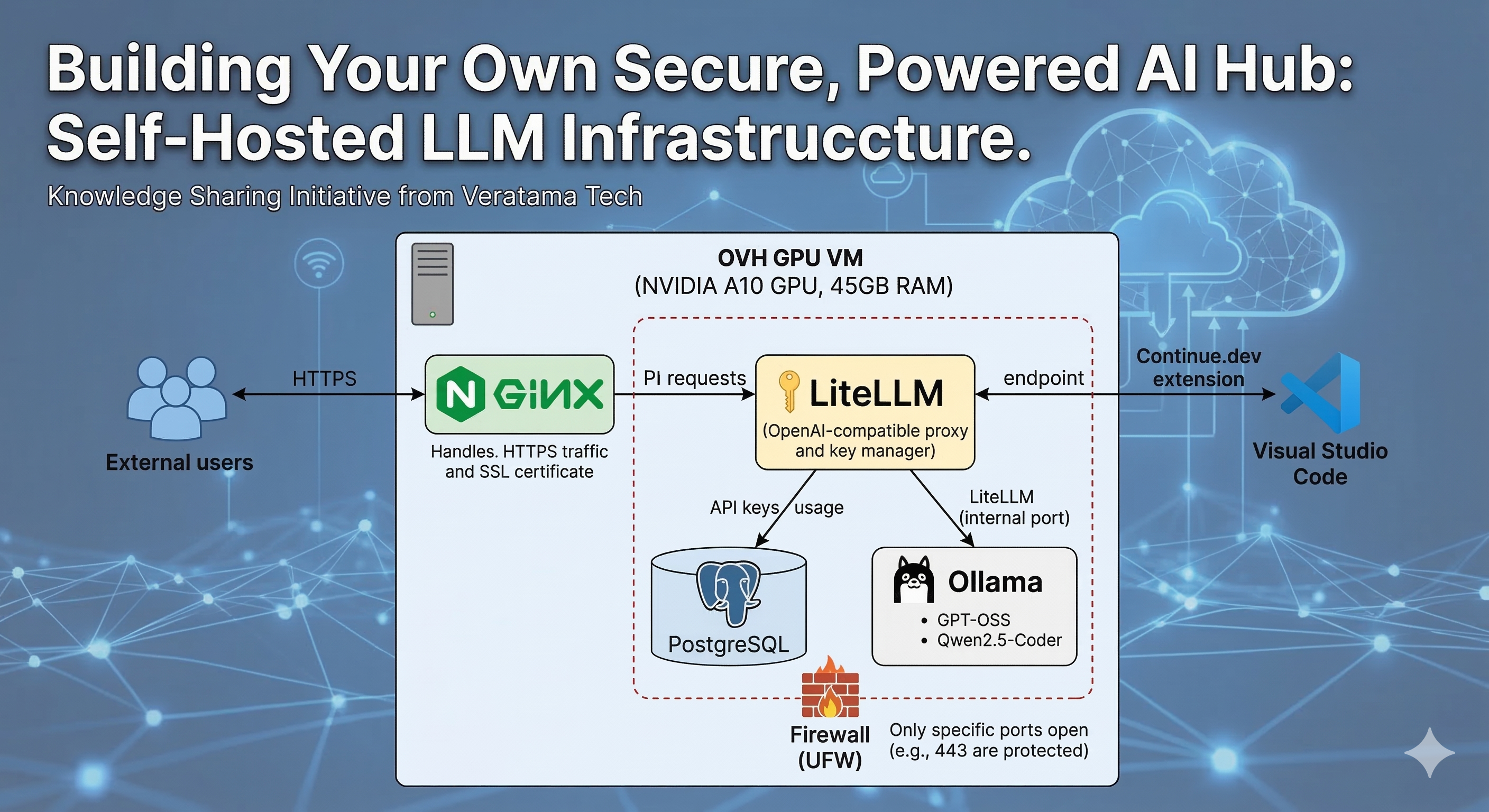

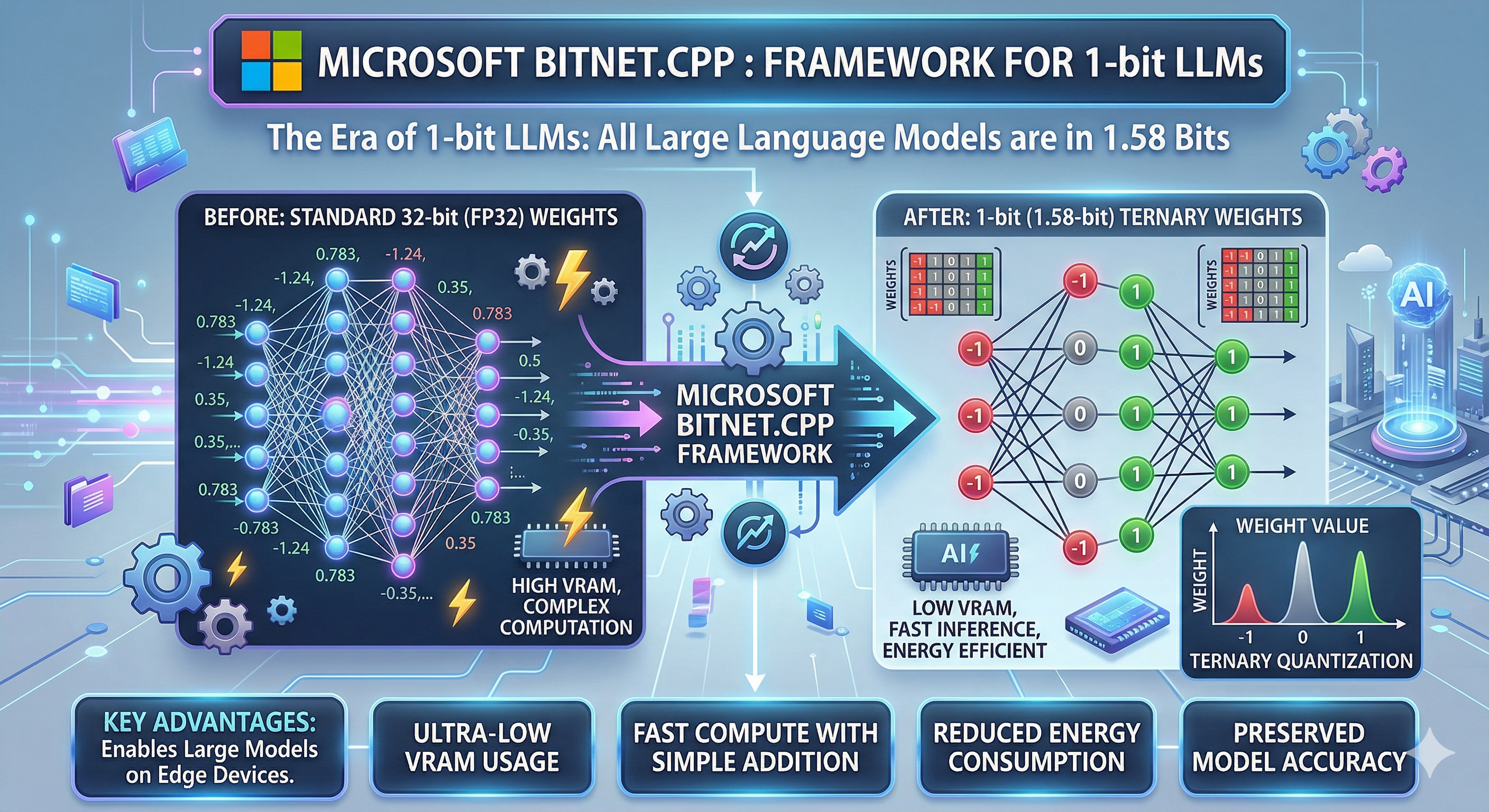











‘0’ Komentar
Tinggalkan Komentar